This chapter introduces some of the main elements required to develop models and explore their behavior. The development of a model amounts to the articulation of hypotheses pertaining to a system under study. One (but not the only one) of the main interests in developing models is to 'see' how the system would behave, assuming that the representation we make of that system is correct.
Here, we use the STELLA® program, because it (almost) directly uses Forrester's symbols, and because we do not have to bother about the syntax of the program. We do have, however, to be consistent with respect to the syntax of Forrester's symbols, which one can consider as pictograms, each of them corresponding to individual computing steps (see previous section). As will be shown in the following text, the choice of this programming platform sets us free from computing details, and instead allows focusing at the system at hand, its time and space characteristics, the way we would like to represent it, and then on the set of equations we believe govern its functioning.
Essentially, STELLA® operates in five stages:
- draw the elements and relationships that represent the structure of the model (this implies choices described in the previous chapter, including the state variables themselves, their dimensions, and the limits of the system);
- decide on a time frame, a time step, and an integration procedure;
- devise equations that relate the state variables, the rates, and the parameters of the model among themselves;
- run the model, and see the outputs as graphs or tables; and
- check the program corresponding to the model which has been developed.
These different stages are linked in different windows of the same STELLA® file.
Exponential growth
In the previous chapter, exponential growth was used as an example for integration, both analytical and numerical. Here, we shall first model exponential growth with the same hypotheses as in the previous chapter: (1) there are no limits to growth (i.e., unlimited supply of nutrients, no self-toxicity), and (2) the rate of growth is constant over time.
One first has to use a state variable, the amount of bacteria, A. A state variable is represented by a box. The next component of the system is a flow of bacterial growth governed by a rate of growth, RA (the number of new bacteria formed per time step). This is represented under STELLA® by a double arrow and a valve. The third element of the system is the relative rate of growth (the number of new bacteria formed per bacterium per time step), RRA. RRA is a parameter (in this example a fixed-value parameter) represented by a circle.
The system also involves relationships among some of its components, that is, flows of information. These relationships concern the effect of RRA on RA (i.e., we state that: 'RA depends on RRA'), and the effect of A on RA (we state that: 'RA also depends on A'). These relationships are represented by simple arrows.
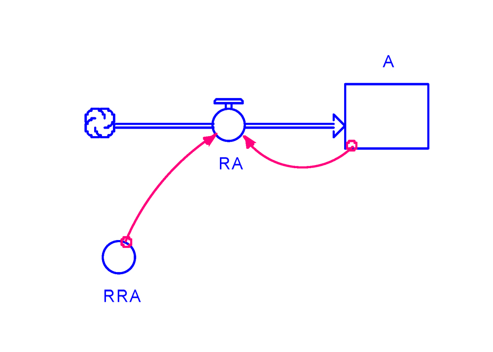
Figure 3.1. A flowchart representing exponential growth.
The flowchart is shown in Fig. 3.1. This very simple drawing therefore says that the amount of bacteria, A, grows with a rate RA, which depends on both the current number of bacteria A and a relative (or 'intrinsic') rate of increase, RRA.
The model corresponding to this diagram then needs documentation. Let us for instance assume that the initial number of bacteria is 1 (i.e., A0 = 1), and that the relative rate of bacterial increase is 0.3, that is, that each bacterium produces 0.3 new bacterium per time step, Δt.
The time characteristics of the system need then to be specified. We may, for instance assume that one is dealing with a 24-h experiment, and that the bacterium population is monitored on an hourly basis. One would, then run the simulation with a time step of Δt = 1 h over a period of time of 24 h.
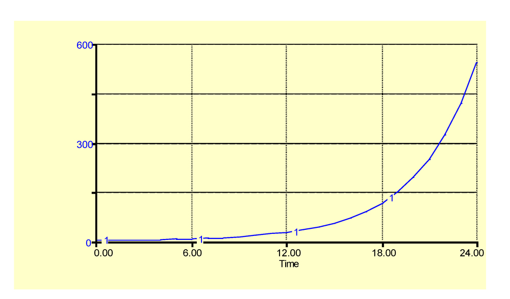
Figure 3.2. Simulated exponential growth. Horizontal axis: time (hours); vertical axis: number of bacteria.
The result is shown in Fig. 3.2, where t is the abscissa and A is the ordinate, with the expected exponential number of bacteria increasing over time.
As a last step, we need to take a look at the program, written for STELLA®, as follows:
A(t) = A(t - dt) + (RA) * dt
INIT A = 1
INFLOWS:
RA = A*RRA
RRA = 0.3
Varying the parameter of exponential growth
The previous paragraph reassures us that we indeed can easily develop a simulation model, even though it admittedly is a very simple one. One question which quickly may arise is whether and to what extent our model is sensitive to its parameter, RRA. To address this question, one can arbitrarily assign to RRA a series of different values, such as: 0.01, 0.05, 0.1, 0.2, and 0.3.
The resulting graph is shown in Figure 3.3. As expected, any incremental increase in the relative rate of increase parameter corresponds to curves that strongly differ not in shapes, but in slopes (speeds) and maxima. This result shows how sensitive the model is to variations of RRA. This does not come as a surprise, of course, but further ensures us that the model does behave as exponential processes do.
Such a simple exercise (analyzing the effects of parameter change on the model output) actually is a sensitivity analysis, used in this case to check whether the program behaves as intended. Sensitivity analysis is a field of its own, with many applications, which we cannot address here.
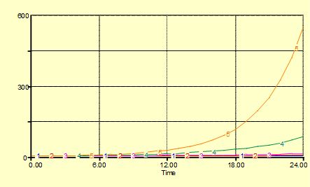
Figure 3.3. Simulated exponential growth with different values of the relative rate of increase, RRA. Curves 1 to 5 correspond to RRA values of 0.01, 0.05, 0.1, 0.2, and 0.3, respectively. Horizontal axis: time (hours); vertical axis: number of bacteria.
Introducing a driving variable: exponential growth with varying relative rate
Until now, we have assumed that the relative rate of increase, RRA, of the exponential process is constant. In many cases, environmental conditions are such that processes involved in a system are influenced. Botanical epidemiology, for instance, provides a wide range of such external influence on the behavior of epidemics.
Still using our exercise exponential model, it is possible to explore ways to see how such external influences may be modeled. Let us for instance assume that RRA varies with temperature, such that, from experimental results, we have the following Table 3.1.
Table 3.1. RRA values according to temperature
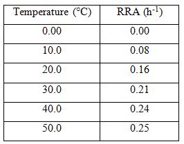
This table indicates that at a temperature of 0°C, RRA is 0, then increases linearly, and then tapers off when temperature approaches 50°C. Instead of a table, this information could be represented by a graph of RRA as a function of temperature. Between each (temperature, RRA) pair of data points, a segment would be drawn, which amounts to a linear interpolation. Many programming languages enable the computation of values that RRA would take according to temperature from such linear interpolations.
Furthermore, let us assume that the experiment was conducted under conditions such that the temperature would have been oscillating around a mean temperature of 20°C with an amplitude of 10°C, which amounts to:
Temp = TempMean + AmpTemp*sin(2*π*time/24)
where Temp is the running temperature, TempMean is the mean temperature, and AmpTemp is the amplitude about which the running temperature varies.
These new elements can be incorporated in the model by adding new components:
- a Temp variable which influences RRA, and
- two driving functions, TempMean and AmpTemp, which, in turn, makes Temp vary.
The model diagram is represented in Fig. 3.4.
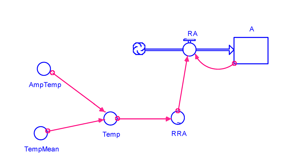
Figure 3.4. A flow chart representing exponential growth with temperature variation as a driving variable.
TempMean and AmpTemp are called driving functions (or driving variables), because they influence the system under consideration externally. If we were strictly using Forrester's symbols, they should be represented by segments with a dot at their center (see previous chapter) in order to indicate that they are different in nature from RRA, which is a parameter inherent to the model under consideration.
The question is whether large variations in RRA, as indicated by the effects of temperature on RRA in the previous table, could strongly influence the behavior of the system. Fig. 3.3 showed how strong the effect of RRA on the model's output can be, and thus one expects a strong response. Under the above assumptions on RRA's response to temperature, and temperature variation over time, one thus expects a strong change in the system's behavior.
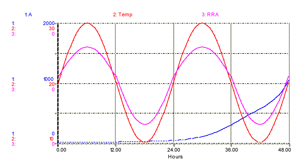
Figure 3.5. Simulation of bacterial numbers (A), temperature (Temp) and relative rate of bacterial increase (RRA). Horizontal axis: time (hours); vertical axis: number of bacteria (A), relative rate of increase of bacterial population (RRA), and temperature (Temp).
Contrary to our initial intuitive reasoning, Fig. 3.5 indicates that the shape of the bacterial population curve is barely influenced by changing temperatures: it still remains an exponential process. Yet, the variations over time of temperature, and of RRA over temperature, are showing the expected sinusoid shapes.
Of course, the values of Table 3.1 were chosen on purpose for this example. We could also have made the amplitude in temperature variation much broader but this would not alter the outcome: what was first designed as an exponential process remains.
The limits to growth - a summarized phytopathological perspective
In a famous report entitled 'The Limits to Growth' to the Club of Rome, Meadows et al. forwarded a grave warning in 1972 to the international community: unlimited growth (as most conventional economists and demographists see it) cannot possibly take place, disregarding the global population growth and the limited resources of the biosphere. This was followed by a series of sequels, including 'Beyond the Limits - Global Collapse or a Sustainable Future' in 1992 (which actually makes extensive use of systems concepts, simulation modeling, and of the STELLA® program), and 'World on the Edge - How to Prevent Environmental and Economic Collapse' in 2011. These warnings have repeatedly been dismissed as simplistic, biased, and Malthusian, because they did not factor in the human ingenuity to solve problems as they emerge. G. Hardin (1968) however made a very strong case in his article on the 'Tragedy of the Commons' in highlighting this particular and (usually extremely important) class of problems which can be called "no technical solution problems".
From a modeler's standpoint, the above example illustrates one of the many uses of simulation modeling. Simulation models enable researchers to conduct (simulation) experiments on systems in which no material experiments could possibly be conducted. There is only one biosphere, and experiments where the rate of, for example, population growth, the amount of available water, the fraction of human beings living in cities, and the amount of food produced per capita would all be varied, are simply unthinkable. Carefully designed models, hypotheses (that is to say, building scenarios), and simulations, as well as cautious interpretations of simulation results, allow us to precisely do that.
Plant disease epidemiologists are confronted with limited growth on a routine basis: a crop has only a limited number of sites (e.g., individual plants, leaves, or fragments of roots, say, per square meter) which may become infected. Once infected, such sites cannot be infected again, and the pathogen is confronted with a limited carrying capacity at each point of time. Epidemics do occur in natural ecosystems too, which are characterized by one among many differences: whereas a crop is to be seen as a cohort of individuals of approximately the same physiological age, and very often, with a similar genetic make-up, host plants in natural ecosystems do not have the same physiological age, and differ genetically. Nevertheless, in both kinds of systems, a limit to (disease) growth exists.
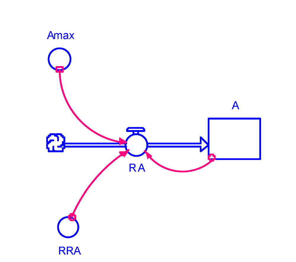
Figure 3.6. Flowchart representing exponential growth with limited growth.
For now, let us return to our simple bacterial model. One important change in the model structure is to consider that bacteria are not growing in an unlimited volume, with unlimited supply of nutrient. We then would introduce the notion of carrying capacity in the model, in this case, represented by the maximum number of bacteria the system might possibly contain. The starting value of the bacterial population was set at 1 (this "1" might represent 1×10⁶ bacteria). Let us now assume that the maximum number of bacteria in the system could only be 100 (or 100×106 bacteria). The model structure then becomes as shown in Fig. 3.6.
Introducing Amax slightly changes the program, as the equation for RA now has to account for Amax, namely, RA is not only function of RRA but is also a (multiplying) function of the distance to which the current bacterial population is far away from reaching its maximum possible value, which we write: (1 - (A/Amax)). This term will be referred to the 'correction factor' in the following chapter. The corresponding modeling program becomes:
A(t) = A(t - dt) + (RA) * dt
INIT A = 1
INFLOWS:
RA = A*RRA*(1 - (A/Amax))
Amax = 100
RRA = 0.3
The resulting bacterial dynamics is shown in Fig. 3.7 with a typical sigmoid curve, with which ecologists, microbiologists, and plant pathologists, are so familiar.
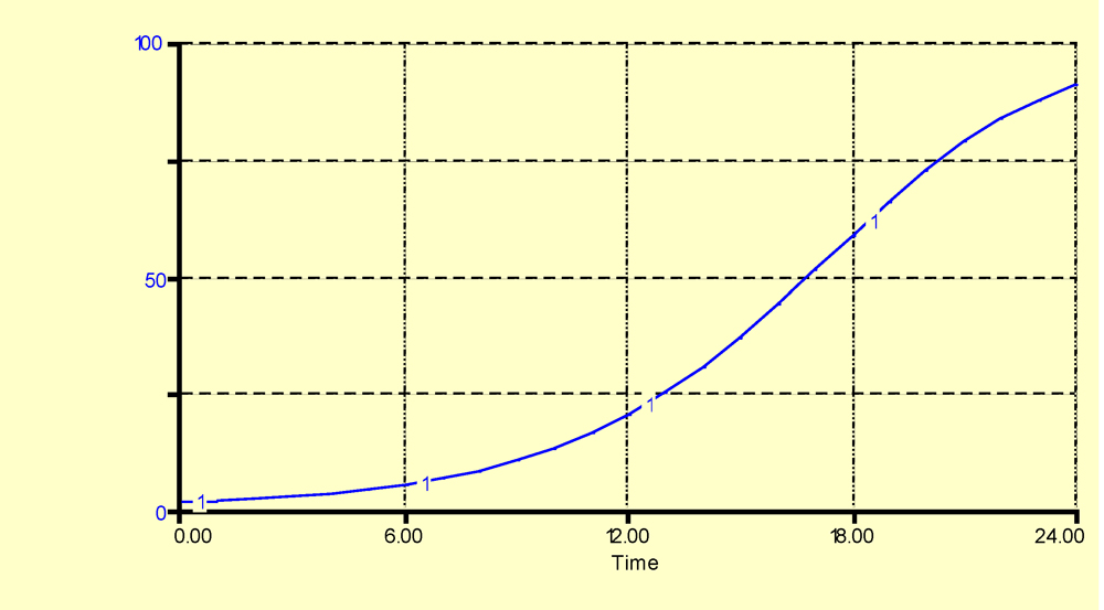
Figure 3.7. Simulated exponential growth with limited growth. Horizontal axis: time (hours); vertical axis: number of bacteria.
Summary
This chapter has introduced some key elements of model development:
- Steps in developing a simulation model including: (1) drawing the relationships representing the model structure; (2) choosing a time frame, a time step, and an integration procedure; (3) running the model, and see the outputs as graphs or tables; and (4) checking the program corresponding to the model which has been developed.
- A very simple system of bacterial growth has been used to illustrate the concepts of rate of growth of a state variable and of relative rate of growth.
- Changes in the value of the relative rate of growth (RRA) have profound consequences in the numerical outcomes of simulations - but not in the shapes of the simulated curves. Varying RRA and assessing the behavior of the system may be seen as a preliminary, qualitative, example of sensitivity analysis.
- The notion of driving function (variable) - of a variable which lies outside the boundaries of the considered system, but may influence it - is introduced. In the bacterial growth example, where the effect of oscillating temperature on RRA is used. Although temperature variation does affect the running value of the rate of growth (RA), it does not truly affect the overall behavior of the system: an exponential process is retained.
- The notions of limited growth and carrying capacity of a system are introduced. This has dramatic consequences on the behavior of the system, and yields a sigmoid growth.
References
Kranz, J. 1988. Measuring plant disease. Pages 35-49 in: Experimental Techniques in Plant Disease Epidemiology. J. Kranz and J. Rotem, eds. Springer Verlag. Berlin, Heidelberg, New York.
Brown, L.R. 2011. World on the Edge - How to Prevent Environmental and Economic Collapse. Earth Policy Institute. W.W. Norton & Company, New York, London.
Forrester, J.W. 1961. Industrial Dynamics. M.I.T. Press, Cambridge (Mass.).
Hardin, G. 1968. The tragedy of the commons. Science 162:1243-1248.
Leffelaar, P.A., ed. 1993. On Systems Analysis and Simulation of Ecological Processes. Current Issues in Production Ecology. Kluwer Academic Publishers, Dordrecht.
Meadows, D.H., Meadows, D. L., Randers, J., and Behrens, W.W. III 1972. The Limits to Growth: A Report to The Club of Rome.
Meadows, D.H., Meadows, D. L., and Randers, J. 1992. Beyond the Limits - Global Collapse or a Sustainable Future. Earthscan, London.
Penning de Vries, F.W.T., and Van Laar, H.H., eds. 1982. Simulation of Plant Growth and Crop Production. Pudoc, Wageningen.
de Wit, C.T., and Goudriaan, J.G. 1978. Simulation of Ecological Processes. Pudoc, Wageningen.
Suggested reading
Case, J.T. 2000. An Illustrated Guide to Theoretical Ecology, Oxford University Press, New York.
Exercises and questions
-
The rate of growth in case of the exponential growth of a variable N is
a. RG = r × N × (1-(N/Nmax))
b. RG = r × N2
c. RG = r × N-1
d. RG = r × N
-
Increasing the relative rate of growth in case of the exponential growth of a variable N
a. Does not affect the dynamics of N
b. Increases the rate of growth
c. Increases the final value of N
d. Decreases the rate of growth
-
A driving function
a. Can be constant over time
b. Corresponds to processes simulated within the system
c. Can vary over time
d. Does not affect the system modeled
-
The rate of growth in case of the exponential growth of a variable N with a carrying capacity Nmax is
a. RG = r × N × (1-(N/Nmax))
b. RG = r × N × (1 – N)
c. RG = r × N-1
d. RG = r × N × (1+(N/Nmax)
-
The dimension of the relative rate of growth of a variable N having an exponential growth is
a. [N.T-1]
b. [N.N-1.T-1]
c. [N.N-1]
d. does not change if the equation of the rate of growth includes a carrying capacity
Answers to exercises and questions
- d: RG = r × N
- b: Increases the rate of growth, and c: Increases the final value of N.
- a: Can be constant over time, and c: Can vary over time
- a: RG = r × N × (1-(N/Nmax))
- b: [N.N-1], and d: does not change if the equation of the rate of growth includes a carrying capacity
