Suppose you are working with a simple system in which precipitation and temperature are the main predictors of disease severity. This might be the case if other potential predictors tend to be fairly constant or tend to stay within the disease-conducive range. (One key to developing a good predictive model is determining what the limiting factors are for disease development.)
The relationship between precipitation, temperature and disease severity could take many forms. If the goal is to predict disease severity over time as a function of weather variables over time, one approach would be to model the rate of change in disease severity or pathogen populations as a function of the weather variables. But before adding environmental effects, let's review logistic growth.
Logistic growth with a constant growth rate
If the discrete logistic curve describes disease progress over time, then the rate of increase is the parameter R in the following equation
Dt+1=Dt+R*Dt*[(1-Dt)/100)]
where Dt indicates the percentage infection at time t and R indicates the growth rate. (See Sparks et al. (2008) for examples of logistic modeling using R in continuous time and Donovan and Weldon's (2002) Chapter 8 for examples in discrete time using Excel.) A series of percentage infection values can be generated in the R programming environment by the following commands.
# Assign a value to the rate parameter R
rate <- 1

# Determine how many time steps, nweeks, will be considered
nweeks <- 10

# Set up a matrix that will contain the percent infection over
#    time
perinf <- matrix(0,nweeks,1)

# Assign the starting value to the first percent infection
#    observation
perinf[1] <- 1

# Generate the percent infection for the following weeks
for (j in 2:nweeks) {
  perinf[j] <- perinf[j-1] * (1 + rate*(1 - perinf[j-1]/100))
}

# plot the time series of percent infection
plot(1:nweeks, perinf, xlab='Time (weeks)',
     ylab='Percent infection', ylim=c(0,100),
     type='l', col='orange')
Output
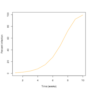
Click to enlarge.
Sparks et al. (2008) give examples of how different values of the rate parameter affect growth over time. In those examples, the rate parameter was assumed to be constant over time. But we can modify the model to make the rate parameter vary at each time point as a function of weather variables
Dt+1=Dt+Rt*Dt*[(1-Dt)/100)]
.
What are some realistic possibilities for the relationship between weather and the rate parameter?
One simple scenario would be that the rate parameter takes on either the value 0 if no precipitation occurs during the preceding week or the value R if precipitation does occur during the preceding week.
Rt = R if precipitation occurs during week t, and Rt = 0 if precipitation does not occur during week t.
Under that scenario, what would disease progress be for different patterns of precipitation?
The model can be made one step more complicated by including temperature as a predictor. Suppose precipitation has the same effect as described above; that is, the presence of a precipitation event makes infection possible. But suppose also that the temperature will affect the rate Rt during those weeks in which precipitation occurs. Perhaps the effect of temperature on the rate of disease progress can be expressed by a simple relationship over the range of temperatures of interest, such as
Rt = R * [1 + ( Tt - 20)/20]
where
Tt indicates the temperature at time
t. (In reality, a straight line relationship like this would probably only describe the relationship over a fairly narrow range of temperatures.) Then combining the precipitation and temperature effects gives
Rt = R * [1 + ( Tt - 20)/20]
if precipitation occurs during week t, and
Rt = 0 if precipitation does not occur during week t.
To visualize this relationship, try the following command.
curve(1 + (x-20)/20,
      from=0,
      to=40,
      xlab='Temperature',
      ylab='R'
)
Simulating rain events
We can simulate the occurrence of precipitation using a draw of a binomial random variable each week. One binomial random variable with mean 0.5 can be generated with the following R command.
rbinom(n=1,size=1,prob=.5)
Here n is the number of variables to be drawn, size is the number of trials that go into determining each variable, and prob is the probability of success, in our case the probability that precipitation occurs. (The binomial distribution can also be used to generate the number of successes out of more than one trial, but here we only have one trial at a time.) We can generate a series of variables indicating whether precipitation occurred for each of nweeks weeks with the following commands.
nweeks <- 10
rprob <- .5
rain <- matrix(0,nweeks,1)
for(j in 1:nweeks){rain[j] <- rbinom(n=1,size=1,prob=rprob)}
rain
Try this set of commands for different values of nweeks and rprob to get a feel for how it works.
Simulating a temperature time series
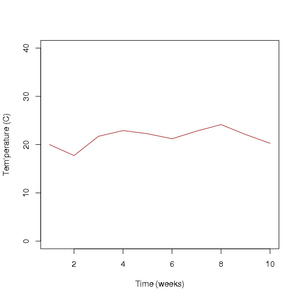
It would be simplest if we could simulate weekly temperatures independently, but that is probably not realistic. Suppose that the correlation in temperature between weeks extends one week into the past, a better approximation. Then, given the temperature in week t, we can generate the temperature in week t+1 by adding a random variable to the earlier temperature. For example, if the temperature in week t was 20° C, the temperature in week t+1 might be generated by adding to 20 a random normal variable with mean zero and standard deviation 2. Try the following command several times to see a range of possible outcomes
20 + rnorm(n=1,mean=0,sd=2)
A series of temperatures can be generated in this way using the R code below. Series like this in which stochastic changes are added to the pre-existing values are sometimes referred to as random walks. Again, try pasting these commands several times to see a range of outcomes.
nweeks <- 10
tempmean <- 20
tempsd <- 2
temp <- matrix(0,nweeks,1)
temp[1] <- 20
for(j in 2:nweeks){
  temp[j] <- temp[j-1] + rnorm(n=1,mean=0,sd=tempsd)
}
plot(1:nweeks, temp, xlab='Time (weeks)',
     ylab='Temperature (C)', ylim=c(0,40),
     type='l', col='brown')
Here is one realization of the series of temperatures generated by this code.
Click to enlarge.
Generating disease progress
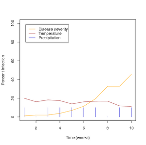
Now we use weather events to generate disease progress. This process is essentially the same as illustrated for logistic growth above except for the added step of adjusting the rate of progress each week based on the weather variables.
# Assign a value to the rate parameter R
# Now this indicates the rate of disease progress
#   under conducive conditions
rate <- 1
# Determine how many time steps, nweeks, will be considered
nweeks <- 10
# Set up a matrix that will contain the percent infection
#   over time
perinf <- matrix(0,nweeks,1)
# Assign the starting value to the first percent infection
#   observation
perinf[1] <- 1
# Generate the series indicating whether rain occurred
rprob <- .5
rain <- matrix(0,nweeks,1)
for (j in 1:nweeks){rain[j] <- rbinom(n=1,size=1,prob=rprob)}
# Generate the series of temperatures
tempmean <- 20
tempsd <- 2
temp <- matrix(0,nweeks,1)
temp[1] <- 20
for(j in 2:nweeks){
  temp[j] <- temp[j-1] + rnorm(n=1,mean=0,sd=tempsd)
}
# Generate the time series of rates
rateseries <- rate * rain * (1 + (temp - 20)/20)
# Generate the percent infection for the following weeks
# Now the constant rate is replaced by a varying rate
for (j in 2:nweeks) {perinf[j] <- perinf[j-1] *
  (1 + rateseries[j-1]*(1 - perinf[j-1]/100))}
# Plot the time series of percent infection
plot(1:nweeks, perinf, xlab='Time (weeks)',
     ylab='Percent Infection OR Temperature',
     ylim=c(0,100), type='l', col='orange')
# Add lines to indicate weeks when precipitation occurs
lines(1:nweeks, rain*10, type='h', col='mediumblue')
# Add a line to indicate temperature
lines(1:nweeks, temp, type='l', col='brown')
# Add a legend
legend('topleft',
       c('Disease severity', 'Temperature', 'Precipitation'),
       lty=c(1,1,1),
       col=c('orange','brown','mediumblue'), inset=0.05)
Output: Example of one realization
Click to enlarge.
Evaluating how often disease severity reaches important thresholds
Now we can ask questions about how frequently disease severity would reach a particular critical level as a function of the typical weather conditions (where the weather parameter rprob, the probability of rainfall in any given week, is set to be adjustable in calls to the new function discast). This will be simpler if the above commands are combined into a function.
discast <- function(rate,nweeks,start,rprob){
# rate is the increase in disease under conducive conditions
# nweeks is the number of weeks being considered
# start is the starting infection percentage
# rprob is the probability of rain in any given week
  perinf <- matrix(0,nweeks,1)
  perinf[1] <- start
  rain <- matrix(0,nweeks,1)
  for (j in 1:nweeks){rain[j] <- rbinom(n=1,size=1,prob=rprob)}
  tempmean <- 20
tempsd <- 2
temp <- matrix(0,nweeks,1)
temp[1] <- 20
for(j in 2:nweeks){
  temp[j] <- temp[j-1] + rnorm(n=1,mean=0,sd=tempsd)
}
# Generate the time series of rates
rateseries <- rate * rain * (1+(temp - 20)/20)
for (j in 2:nweeks) {
  perinf[j] <- perinf[j-1] *
     (1 + rateseries[j-1]*(1 - perinf[j-1]/100))
}
# keep the final infection level as output
  perinf[nweeks]
}
Using this function, we can collect the final infection level for 1000 simulations and evaluate a histogram of the final infection levels.
# set up a matrix to contain the outcome of each simulation
outinf <- matrix(0,1000,1)
# run the function discast 1000 times
for (j in 1:1000){
  outinf[j] <- discast(rate=1,nweeks=10,start=1,rprob=.5)}
# plot the histogram of final disease levels
hist(outinf,xlim=c(0,100),col='dark blue')
Output
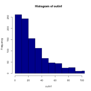
Click to enlarge.
The construction of the histogram can also be formulated as a function to make it easier to examine the results for different parameter values for rate, nweeks, etc.
comp <- function(ratein=1, nweeksin=10, startin=1, rprobin=.5){
  outinf <- matrix(0,1000,1)
  for (j in 1:1000){
    outinf[j] <- discast(rate=ratein, nweeks=nweeksin,
                         start=startin, rprob=rprobin)
  }
  hist(outinf, xlim=c(0, 100))
}
If you run the same set of parameter entries over and over, how does the shape of the histogram change? Try exploring the results for different parameter values. For example, how often does disease severity exceed 30% for each parameter combination you test?
comp(ratein=0.5,nweeksin=15,startin=1,rprobin=.3)
The effects of an intervention on disease progress
Suppose an intervention such as a pesticide application is used to reduce the rate of disease progress, and it reduces the rate of disease progress by a proportion I during the week when it is applied. The effect might be incorporated by adding another step to the simulation.
|
Rt |
Precipitation occurs |
Intervention |
|
I * R * (Tt - 20)/20 |
Yes |
Yes |
|
R * (Tt - 20)/20 |
Yes |
No |
|
I * 0 |
No |
Yes |
|
0 |
No |
No |
Constructing a decision rule for applying an intervention
There are at least two types of uncertainty in the weather series that complicate decisions about whether to use an intervention. First, the rules determining the generation of weather and the relationship between weather and disease are not really known and have to be estimated from limited data. Second, even if the rules were known, there is still a stochastic part to the generation of weather patterns (or is there?). If you observed the patterns of weather and the relationships between weather and disease that we illustrate here, what type of decision rule might you construct?
The construction of the rule would depend at least in part on the level of disease severity that results in yield loss, Y. If the cost of the intervention is negligible (not often the case), then the intervention would provide economic benefits if it keeps the disease level below the yield loss threshold. A rule might be of the form:
Rule 1: Apply intervention if disease severity is greater than Y-10.
Note that the value 10 provides a buffer so that the intervention application is called for before the economic threshold is actually reached. (One research goal might be to determine whether 10 or another value would be a better buffer.)
We can test how well this rule works by adjusting the generation of disease progress to include the intervention. We could add more parameters to the function, but instead let’s assume that the effect of the intervention is to multiple the rate of disease increase by the proportion 0.1 and that the threshold level of disease severity is 40%.
discast <- function(rate,nweeks,start,rprob,inter){
  # rate is the increase in disease under conducive conditions
  # nweeks is the number of weeks being considered
  # start is the starting infection percentage
  # rprob is the probability of rain in any given week
  # inter indicates whether the intervention rule will be used
  #   or not
  perinf <- matrix(0, nweeks, 1)
  perinf[1] <- start
  rain <- matrix(0, nweeks, 1)
  for (j in 1:nweeks){
    rain[j] <- rbinom(n=1,size=1,prob=rprob)
  }
  tempmean <- 20
  tempsd <- 2
  temp <- matrix(0,nweeks,1)
  temp[1] <- 20
  for(j in 2:nweeks){
    temp[j] <- temp[j-1] + rnorm(n=1,mean=0,sd=tempsd)
  }
  rateseries <- rate * rain * (1 + (temp - 20)/20)
  for (j in 2:nweeks) {
    trate <- rateseries[j-1]
    if(perinf[j-1] > 40-10 & inter) {
      trate <- 0.1*trate
    }
    perinf[j] <- perinf[j-1] *
        (1 + trate*(1 - perinf[j-1]/100))
  }
  # keep the final infection level as output
  perinf[nweeks]
}
Now try running many simulations as above, comparing the results with and without the intervention. The intervention is applied following the rule when the variable inter is set to T in the call to the new function discast.
# set plot area for two histograms
par(mfrow=c(2,2))

# set up a matrix to contain the outcome of each simulation
outinf <- matrix(0,1000,1)
# run the function discast 1000 times with intervention
for (j in 1:1000){
  outinf[j] <- discast(rate=1, nweeks=10, start=1, rprob=.5,
                       inter=T)
}
# plot the histogram of final disease levels
hist(outinf, xlim=c(0, 100), col='dark blue',
     main='With Intervention')

# set up a matrix to contain the outcome of each simulation
outinf <- matrix(0,1000,1)
# run the function discast 1000 times with out intervention
for (j in 1:1000){
  outinf[j] <- discast(rate=1, nweeks=10, start=1, rprob=.5,
                       inter=F)
}
# plot the histogram of final disease levels
hist(outinf, xlim=c(0, 100), col='light green',
     main='With Out Intervention')
Output
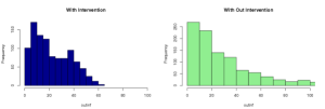
Click to enlarge.
How frequently does lack of intervention result in high levels of infection?
Next, a simple generic infection model example
