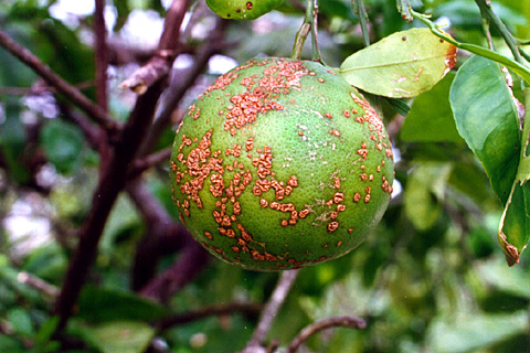
Citrus canker symptoms on fruit: Citrus canker, caused by Xanthomonas axonopodis pv. citri, on grapefruit.
For this exercise, it is recommended that you have Gottwald et al. (1989) on hand while reading this section and doing the exercises. There are some key points illustrated in the paper that are not presented here.
Bacterial colonization of host plants requires the entry of the pathogen into host tissues, most commonly through natural openings in the plant such as stomata, lenticels, or wounds on the plant surfaces (Vidaver and Lambrecht 2004). However, pathogen entry can also be achieved through deposition by insects or mechanically through a larger carrier. Bacteria primarily rely on wind or water (splash) dispersal in order for populations to move to new hosts. When rain is driven by significant winds, the rate of disease progress typically increases (Gottwald 2000). High winds tend to result in plant surface abrasion and wet conditions usually result in open stomata, both promoting the entry of the pathogen into its host.
Xanthomonas axonopodis is the casual agent of citrus bacterial canker (CBC). There are three main classifications of CBC within the species, the most prevalent of which is Asiatic CBC caused by X. axonopodis pv. citri (Xac). When infected with Xac, a host plant will exhibit lesions on leaves, stems, and fruits. The disease induces early leaf and fruit abscission, resulting in tree health decline. Infection with Xac renders any infected fruit unsalable, explaining the economic importance of controlling this pathogen.
To illustrate how disease progress over time occurs for a bacterial pathogen, consider the example of Gottwald et al. (1989). Several models were compared for describing the progression of citrus CBC on three citrus crops in a nursery setting using two methods of data collection (Gottwald et al. 1989). The details for the experimental design and objectives may be found in the paper. In this exercise, R will be used to illustrate the visual comparison of different disease progress curves.
Because previous research had related disease spread to wind-driven rain, Gottwald et al. (1989) were interested in the effect that this phenomenon would have in a densely-planted nursery setting. Figure 1 from Gottwald et al. (1989) depicts both disease incidence and rainfall, but the occasions where rainfall was associated with heavy winds (>8 ms-1) are indicated by arrows. This is consistent with the idea of a direct relationship between disease progress in the nursery and the occurrence of wind-driven rain.
Gottwald et al. (1989) considered a number of models including the exponential, monomolecular, Gompertz, logistic, and Weibull, to describe disease progress in each nursery using both disease incidence and disease severity. Table 1 from Gottwald et al. (1989) shows each of these models and depicts how well each of them fit each nursery data. While scrutinizing Table 1, notice several different models do a good job of predicting disease incidence and disease severity over time.
Next, we use R to illustrate the models appliced in Gottwald et al. (1989), we use R to examine the different disease progress curves and compare how well the different models fit the data.
Plotting two exponential curves
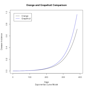
This example illustrates a graphical comparison of two exponential curves using orange and grapefruit parameter estimates derived from Table 1 in Gottwald et al. (1989).
y1 and y2 represent initial infection (at time zero), determined by dividing the number of infected trees by the total number of trees in each respective plot.
r1 and r2 represent the parameters estimated by Gottwald et al.
max1 and max2 represent the number of days disease was studied for each crop.
##Set up function
plot2 <- function(y1,y2,r1,r2,max1,max2){
  # The first curve
  curve(
          y1*exp(r1*x),
          from=0,
          to=max1,
          add=FALSE,
          lty=1,
          xlab='Days',
          ylab='Disease Incidence',
          col='black',
          xlim=c(0,400),
          ylim=c(0,1)
  )
  # The second curve
  curve(y2*exp(r2*x),
          from=0,
          to=max2,
          add=TRUE,
          lty=1,
          col='mediumblue'
  )
}
##Run the function plot2
plot2(0.0017,0.0017,0.01579,0.01661,383,382);
##Creates title for the graph and subtitle at bottom
title(main="Orange and Grapefruit Comparison",
  sub="Exponential Curve Model")
##Creates legend in upper left corner
legend(
  "topleft",
  c("Orange","Grapefruit"),
  lty=c(1),
  col=c("black","mediumblue"),
  inset=0.05
)
Output

Click on the image for larger version.
Plotting three exponential curves.
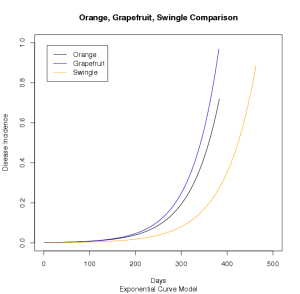
This example illustrates how to plot three exponential curves for comparison using orange, grapefruit, and swingle parameter estimates derived from Table 1 in Gottwald et al. (1989).
##Set up function
plot3 <- function(y1,y2,y3,r1,r2,r3,max1,max2,max3){
  # The first curve
  curve(y1*exp(r1*x),
          from=0,
          to=max1,
          add=FALSE,
          lty=1,
          xlab='Days',
          ylab='Disease Incidence',
          col='black',
          xlim=c(0,500),
          ylim=c(0,1)
  )
  # The second curve
  curve(y2*exp(r2*x),
          from=0,
          to=max2,
          add=TRUE,
          lty=1,
          col='mediumblue'
  )
  # The third curve
  curve(y3*exp(r3*x),
          from=0,
          to=max3,
          add=TRUE,
          lty=1,
          col='orange'
  )
}
##Run the function plot3
plot3(0.0017,0.0017,0.001,0.01579,0.01661,0.01466,383,382,463);
##Creates title for the graph and subtitle at bottom
title(
  main="Orange, Grapefruit, Swingle Comparison",
  sub="Exponential Curve Model"
)
##Creates legend in upper left corner
legend(
  "topleft",
  c("Orange","Grapefruit","Swingle"),
  lty=c(1),
  col=c("black","mediumblue","orange"),
  inset=0.05
)
Output

Click on the image for larger version.
Suggested Exercise
Now that you have experience plotting two and three curves on a single graph for the exponential model, use examples two through five to create monomolecular, logistic, Gompertz, and Weibull curves of disease incidence using the following parameter estimates.
TABLE 1: Disease progress parameter estimates from Gottwald et al. (1989).
| Model |
Nursery |
Parameter |
Estimate |
| Exponential |
Orange |
r |
0.01579 |
| Exponential |
Grapefruit |
r |
0.01661 |
| Exponential |
Swingle |
r |
0.01466 |
| Monomolecular |
Orange |
r |
0.00180 |
| Monomolecular |
Grapefruit |
r |
0.00242 |
| Monomolecular |
Swingle |
r |
0.00097 |
| Logistic |
Orange |
r |
0.01787 |
| Logistic |
Grapefruit |
r |
0.02047 |
| Logistic |
Swingle |
r |
0.01636 |
| Gompertz |
Orange |
k |
0.02922 |
| Gompertz |
Grapefruit |
k |
0.03179 |
| Gompertz |
Swingle |
k |
0.02860 |
| Weibull |
Orange |
b |
359.27 |
|
|
c |
12.23 |
| Weibull |
Grapefruit |
b |
331.10 |
|
|
c |
10.04 |
| Weibull |
Swingle |
b |
428.05 |
|
|
c |
12.27 |
Next, modeling cassava mosaic disease using growth curves.
