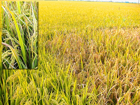
Bacterial blight of rice caused by Xanthomonas oryzae pv. oryzae in a South Korea research station field, showing affected leaves in inset. Photo courtesy F. White, Kansas State University, Manhattan, Kansas.
Bacterial blight of rice causes annual losses as high as 60%. This disease is caused by Xanthomonas oryzae pv. oryzae, a gram-negative, non-spore-forming rod-shaped bacterium. The symptoms manifest as large yellowish lesions extending from the tip of the leaves to the base. The lesions become powdery white as the infection progresses. The pathogen enters the plant through natural openings like hydathodes or through wounds. Bacterial blight epidemics are most common during the heavy monsoons that occur seasonally in south Asia and India (Mew et al. 1993). These heavy rains cause water runoff from infected fields, thereby spreading the pathogen and disease to adjacent healthy fields. Epidemics are often observed following typhoons as a result of severe winds that damage the rice plants, causing wounding, and as the result of wind blown rain that disseminates bacteria over long distances (Nino-Liu et al. 2006). More information about bacterial blight of rice may be found on the International Rice Research Institute (IRRI) Bacterial Leaf Blight Page.
The objective of Mundt et al. (1999) was to measure the dispersal potential of X. oryzae pv. oryzae using experimental plots at IRRI, Philippines, during the wet seasons of 1994 and 1995. Plants within individual hills were clip inoculated to provide the inoculum source within an experimental plot. The plots experienced more than one typhoon during the period of study. Plots were inoculated three times (early tillering, mid tillering and late tillering stages) in 1994 and just once (early tillering) in 1995. In both years lesion counts were made 30 to 35 days after inoculation. The data obtained were analyzed using two different models – the Modified Gregory model (modified power law, y=a(s+c)-b) and Kiyosawa & Shiyomi model (exponential model).
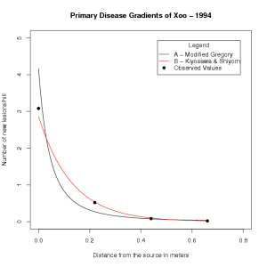
The Gregory model and Kiyosawa & Shiyomi model described similar trends, with steep dispersal gradients in both years of the study. Mundt et al. (1999) concluded that splash dispersal of X. oryzae pv. oryzae was the primary mechanism for such a steep gradient. Furthermore, Mundt et al. (1999) concluded that the Kiyosawa and Shiyomi model provided a superior fit to the observed data.
To examine the dispersal gradients from Mundt et al. (1999) try the following R code,
for 1994 (Figure 1 in the paper):
#Modified Gregory parameter estimates - 1994
a <- 0.01703
c <- 0.11
b <- 2.492

#Kiyosawa & Shiyomi parameter estimates - 1994
A <- 2.867
d <- 7.650

#max is the maximum distance considered - 1994
max <- 0.66

#Modified Gregory Curve
curve(a*(x+c)^(-b),
from=0, to=max,
add=FALSE,
lty=1,
xlab='Distance from the source in meters',
ylab='Number of new lesions/hill',
col='black',axes=TRUE,
ylim=c(0,5),
xlim=c(0,0.8),
main='Primary Disease Gradients of Xoo - 1994')

#Kiyosawa & Shiyomi Curve
curve(A*exp(-d*x),
from=0,
to=max,
add=TRUE,
lty=1,
col='red')

#y contains the number of new lesions
y <- c(3.083,0.521,0.083,0.021)

#y2 contains the distances studied (meters)
y2 <-c (0.0,0.22,0.44,0.66)

#Plot the observed points
points(y2,y,pch=19,col='black')

#Position the legend of the graph in upper left corner
legend('topright',
c('A - Modified Gregory',
  'B - Kiyosawa & Shiyomi',
  'Observed Values'),
lty=c(1,1,NA),
pch=c(NA,NA,19),
col = c('black','red','black'),
title='Legend',
inset=0.05)
Output

Click on the image for larger version.
Suggested exercise
For 1995, similar plots may be made using the 1994 code with the following modifications for the parameters and raw data. How does this plot compare to 1995?
#Modified Gregory Variables - 1995
a <- 0.02622
c <- 0.11
b <- 2.738

#Kiyosawa & Shiyomi Variables - 1995
A <- 7.684
d <- 8.553

max <- 0.66

#This sets the y for observed data
y <- c(7.185,1.380,0.157,0.028)

#This positions the points on the X axis (meters)
y2 <- c(0.0,0.22,0.44,0.66)
