DisplayTitle

Case Study #2: Primary and Secondary Gradients

Septoria leaf spot, caused by Septoria lycopersici on greenhouse tomato. Photo courtesy M. Bates, Kansas State University, Manhattan, Kansas.

Septoria leaf spot, caused by Septoria lycopersici, infects solanaceous species, including many weeds. Conidia are spores borne in pycnidia and these spores may infect tomato plants at any developmental growth stage, but controlling new infections is most critical around the time of anthesis. Infection typically occurs first within the bottom leaves of the tomato plant and then progresses upward. The leaf spotting leads to leaflet necrosis and leaf abscission. This loss of leaves renders tomato fruit susceptible to sunscalding, and puts the plant in an unfavorably stressed condition. Both of these factors contribute to the economic importance of this fungal pathogen.

Because S. lycopersici is both parasitic and saprophytic, managing the crop residue is a major method for reducing inoculum from season to season. Weed management is also critical, since S. lycopersici is known to infect weed hosts.

Dissemination of S. lycopersici spores occurs via multiple mechanisms, including, wind-blown water, water-splash, insect transfer, and mechanical transfer (e.g. equipment, humans, etc.), where wind-blown water and/or water-splash are the most important.

As part of a larger study of the epidemiology of Septoria leaf spot, Parker et al. (1997) examined disease gradients of S. lycopersici over two years. In their experiments, a single plant, positioned in the center of 25 plants within a single row was inoculated with S. lycopersici at five (1992) or six (1993) weeks after transplanting. Plants were spaced at 60 cm intervals. Disease severity was assessed as defoliation and this was defined as the number of abscised leaves plus the number of completely necrotic (still attached) leaves. Gradients were measured over time and this enabled a comparison of primary and secondary dispersal/disease gradients.

Parker et al. (1997) observed that gradients became relatively constant three to five weeks after inoculation. The observed gradients reflected secondary foci. Parker et al. (1997) concluded that the logistic model best described the secondary disease gradients for this pathogen.

The following exercise examines the model assumptions for primary and secondary gradients. For many situations where a secondary gradient is measured, the exponential and power law distributions do not reflect the inherent dispersal process. This is because gradients tend to flatten over time as the source of inoculum expands. An extension of the exponential model for secondary gradients is the logistic model. Also, for power law models, an extension for secondary gradients is the use of a power-logistic model. To follow the results of Parker et al., who found that the logistic model best fit most of the disease gradient curves, an example is presented based on data from Figures 1 and 2 of their paper. In this example, disease gradients have been constructed for two sampling dates, where one represents a gradient assessed just after inoculation of the focus, while the second is a gradient for an assessment that occurred approximately three weeks later (assuming 7-day assessment intervals). Table 2 presents the raw data.

Table 2. Percent defoliation (adapted from Parker et al. (1997)) for a single dispersal gradient for tomato plants, where assessment date 1 was just after inoculation of a focus, while assessment date 4 was approximately three weeks later. Percent defoliation included abscised and necrotic leaves.

To examine these two gradients in R, the following code may be used.

#Construct vectors for the distance and defoliation data
distance <- c(60,120,180,240,300,360,420,480,540,600,660)
date1 <- c(75,40,30,20,15,12,10,12,8,5,4)
date4 <- c(87,78,68,62,50,27,32,12,13,5,4)

#Compare the two gradient curves on the same plot
plot(
  distance,
  date1,
  type='b',
  lty=1,
  pch=19,
  col='black',
  ylim=c(0,100),
  xlab='Distance (cm)',
  ylab='Percent defoliation'
)

lines(
  distance,
  date4,
  type='b',
  lty=1,
  pch=20,
  col='red'
)

legend(
  'topright',
  c('Date1','Date4'),
  lty=c(1,1),
  pch=c(19,20),
  col=c('black','red'),
  title='Legend',
  inset=0.02
)

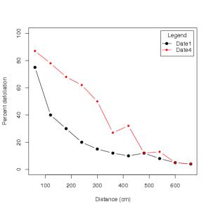
From which the following plot is obtained:

Output

Click on the image for larger version.

It appears that for date four, the percent defoliation is beginning to flatten out, exhibiting a more sigmoidal (S-shaped) curve. This would be expected when secondary dispersal occurs, as newly infected plants also become a source of inoculum for dispersal to longer distances from the original source. Regression analysis may be used to compare which model best fits data from each date.

Suggested exercises

Examine date 1 and date 4 using the power and power-logistic distributions.

Following the methods of Parker

log.date1=log(date1)
log.date1
log.date4=log(date4)
log.date4
logit.date1=log(date1/(100-date1))
logit.date1
logit.date4=log(date4/(100-date4))
logit.date4

Now using the transformed data, linear regression methods in R (Sparks et al. 2008) may be used to compare the two models:

#Set up data frames for each set of regressions
regression1A=as.data.frame(cbind(distance,log.date1))
regression1B=as.data.frame(cbind(distance,logit.date1))
regression4A=as.data.frame(cbind(distance,log.date4))
regression4B=as.data.frame(cbind(distance,logit.date4))

#Perform linear regressions for the four modeling scenarios
dispersal.1A=lm(log.date1~distance,data=regression1A)
dispersal.1B=lm(logit.date1~distance,data=regression1B)
dispersal.4A=lm(log.date4~distance,data=regression4A)
dispersal.4B=lm(logit.date4~distance,data=regression4B)

What information might we want from linear regression? In addition to the methods described in Sparks et al. (200x) for assessing a linear regression fit, some of the summary statistics that provide insight into how well a model fits data include the coefficient of determination (R²), residual mean square error (RMSE), as well as plots of residuals. These may be obtained using the summary function for a linear model.

#For further information on the summary function in R,
#   type ?summary.lm
summary(dispersal.1A)

Call:
lm(formula = log.date1 ~ distance, data = regression1A)

Residuals:
     Min       1Q   Median       3Q      Max 
-0.22791 -0.15540 -0.03715  0.08628  0.35004 

Coefficients:
              Estimate Std. Error t value Pr(>|t|)    
(Intercept)  4.2253264  0.1369926   30.84 1.94e-10 ***
distance    -0.0042979  0.0003366  -12.77 4.53e-07 ***
---
Signif. codes:  0 '***' 0.001 '**' 0.01 '*' 0.05 '.' 0.1 ' ' 1 

Residual standard error: 0.2118 on 9 degrees of freedom
Multiple R-Squared: 0.9477,     Adjusted R-squared: 0.9419 
F-statistic:   163 on 1 and 9 DF,  p-value: 4.535e-07

summary(dispersal.1B)

Call:
lm(formula = logit.date1 ~ distance, data = regression1B)

Residuals:
    Min      1Q  Median      3Q     Max 
-0.4417 -0.2997 -0.1489  0.2100  1.0097 

Coefficients:
              Estimate Std. Error t value Pr(>|t|)    
(Intercept)  0.4343264  0.2946757   1.474    0.175    
distance    -0.0057575  0.0007241  -7.951 2.32e-05 ***
---
Signif. codes:  0 '***' 0.001 '**' 0.01 '*' 0.05 '.' 0.1 ' ' 1 

Residual standard error: 0.4557 on 9 degrees of freedom
Multiple R-Squared: 0.8754,     Adjusted R-squared: 0.8615 
F-statistic: 63.22 on 1 and 9 DF,  p-value: 2.325e-05

summary(dispersal.4A)

Call:
lm(formula = log.date4 ~ distance, data = regression4A)

Residuals:
       Min         1Q     Median         3Q        Max 
-0.3912944 -0.2316225  0.0001519  0.2429178  0.5220735 

Coefficients:
              Estimate Std. Error t value Pr(>|t|)    
(Intercept)  5.1761259  0.2077517   24.91 1.30e-09 ***
distance    -0.0053154  0.0005105  -10.41 2.56e-06 ***
---
Signif. codes:  0 '***' 0.001 '**' 0.01 '*' 0.05 '.' 0.1 ' ' 1 

Residual standard error: 0.3213 on 9 degrees of freedom
Multiple R-Squared: 0.9233,     Adjusted R-squared: 0.9148 
F-statistic: 108.4 on 1 and 9 DF,  p-value: 2.555e-06

summary(dispersal.4B)

Call:
lm(formula = logit.date4 ~ distance, data = regression4B)

Residuals:
     Min       1Q   Median       3Q      Max 
-0.32605 -0.17259  0.02783  0.15084  0.42314 

Coefficients:
              Estimate Std. Error t value Pr(>|t|)    
(Intercept)  2.3814647  0.1658552   14.36 1.65e-07 ***
distance    -0.0084723  0.0004076  -20.79 6.46e-09 ***
---
Signif. codes:  0 '***' 0.001 '**' 0.01 '*' 0.05 '.' 0.1 ' ' 1 

Residual standard error: 0.2565 on 9 degrees of freedom
Multiple R-Squared: 0.9796,     Adjusted R-squared: 0.9773 
F-statistic: 432.1 on 1 and 9 DF,  p-value: 6.457e-09

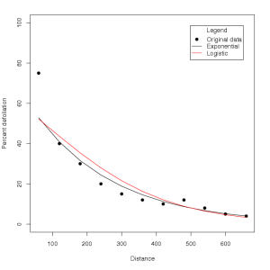
It appears that for date one, the exponential model provides a better fit for the gradient, while for date four, the logistic model provides a better fit. To visually compare the fits of these models with the original raw data, the fitted values for each regression can be backtransformed into the original units (% defoliation) using the following R code:

#The lines below take the fitted value from each
#   regression analysis
#   and backtransforms the data into % defoliation
back.fitted.1A=exp(dispersal.1A$fitted.values)
back.fitted.1B=(exp(dispersal.1B$fitted.values)/
               (exp(dispersal.1B$fitted.values)+1))*100
back.fitted.4A=exp(dispersal.4A$fitted.values)
back.fitted.4B=(exp(dispersal.4B$fitted.values)/
               (exp(dispersal.4B$fitted.values)+1))*100

#The subsequent plots may be created:

plot(
  distance,
  date1,
  type='p',
  pch=19,
  xlab='Distance',
  ylab='Percent defoliation',
  ylim=c(0,100))
  lines(distance,back.fitted.1A,type='l',lty=1,col='black')
  lines(distance,back.fitted.1B,type='l',lty=1,col='red')
  legend('topright',
  c('Original data','Exponential','Logistic'),
  lty=c(NA,1,1),
  pch=c(19,NA,NA),
  col=c('black','black','red'),
  title='Legend',
  inset=0.05
)

which leads to (date 1):

Output

Click on the image for larger version.

#Date 4 Plots:
plot(
  distance,
  date4,
  type='p',
  pch=19,
  xlab='Distance',
  ylab='Percent defoliation',
  ylim=c(0,100))
  lines(distance,back.fitted.4A,type='l',lty=1,col='black')
  lines(distance,back.fitted.4B,type='l',lty=1,col='red')
  legend('topright',
  c('Original data','Exponential','Logistic'),
  lty=c(NA,1,1),
  pch=c(19,NA,NA),
  col=c('black','black','red'),
  title='Legend',
  inset=0.05
)

(date 4):

Output

Click on the image for larger version.

 

Next, Dry-dispersal and rain-splash of brown (Puccinia recondita f.sp. tritici) and yellow (P. striiformis) rust spores from infected wheat leaves exposed to simulated raindrops