DisplayTitle

Case Study #2: Lloyd's Index of Patchiness

Verticillium dahliae is a fungus causing Verticillium wilt in more than 160 plant species including trees, vegetable crops, woody and herbaceous ornamentals. Since 1990, commercial cauliflower has been severely affected by Verticillium wilt. The fungus gains entry via wounds in the roots. The mycelia grow into the vascular system where the fungus reproduces. Eventually the xylem is blocked, preventing water from reaching the leaves. Symptoms associated with the disease on cauliflower are chlorosis, defoliation, stunting, wilting, and vascular discoloration. The pathogen can survive in the soil as microsclerotia for nearly 13 years, making control difficult. The best control methods are to prevent the movement of contaminated soils, plant tolerant cultivars, and eliminate susceptible weed hosts. Since the microsclerotia survive for such long periods of time, crop rotation is not effective.

Xiao et al. (1997) used Lloyd's Index of Patchiness (LIP) to determine the aggregation of microsclerotia. In their analysis, they concluded that all sites had an aggregated spatial distribution of microsclerotia. A beta-binomial distribution was also fit to the wilt incidence data. They concluded that only five out of the 12 sites had an aggregated spatial pattern of wilt incidence, while the other seven sites had a random pattern.

Lloyd's Index of Patchiness was used to determine the level of aggregation. If the LIP estimate is greater than one, this indicates that the pattern is aggregated. As LIP increases, the degree of aggregation also increases. If LIP is less than one, this indicates a random pattern. The following equation can be used to determine LIP for a sample: .

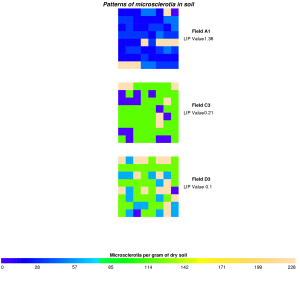
R can be used to calculate LIP for a sample. In our example we use some of the means reported by Xiao et al. (1997) to provide an illustration of their analysis in R. Examples will be shown for data from samples mapped in their fields A1, C3, and D3.

The first step is to download and install the "pixmap" package used to generate the images illustrating the pattern of microsclerotia in the field.

# For this script a special package is required.  This
# command downloads and installs the required "pixmap"
# package.  Select the mirror closest to you when the
# window with a list of mirrors opens.
# This may require root or administrator access
# depending upon your system.install.packages("pixmap")

Now that the pixmap package has been installed, the rest of the R-script can be run.

# Load the newly installed package libraryrequire(pixmap)
# Assign all data points to a vector for A1
A1 <- c(
  23,38,23,38,23,23,23,227,
  23,38,38,38,23,38,23,227,
  23,23,23,38,23,38,23,227,
  53,23,23,38,227,23,38,53,
  53,23,38,23,38,23,23,53,
  23,23,38,53,227,38,23,38,
  227,53,23,38,227,53,23,38,
  7.5,53,53,38,227,38,23,38
)
# Put A1 into the LIP equation
A1.LIP <- round(((mean(A1) + var(A1))/(mean(A1) - 1))/(mean(A1)),
                digits=2)

#for C3
C3 <- c(
  38,7.5,7.5,23,23,23,7.5,23,
  38,23,7.5,23,23,23,7.5,7.5,
  23,7.5,7.5,23,23,23,23,23,
  23,23,23,23,23,23,23,23,
  23,7.5,23,23,23,23,23,23,
  23,23,23,7.5,38,38,23,7.5,
  23,23,38,23,7.5,23,23,7.5,
  38,23,23,23,23,23,23,23
)
# Put C3 into the LIP equation
C3.LIP <- round(((mean(C3) + var(C3))/(mean(C3) - 1))/(mean(C3)),
                digits=2)

#for D3
D3 <- c(
  79,53,38,53,79,53,53,53,
  38,53,38,53,38,38,53,38,
  79,53,79,53,53,53,38,23,
  79,53,53,53,79,53,38,53,
  53,53,38,53,53,53,53,53,
  79,53,79,38,79,38,53,38,
  79,53,38,79,79,53,79,79,
  53,53,53,53,23,79,38,38
)
# Put D3 into the LIP equation
D3.LIP <- round(((mean(D3) + var(D3))/(mean(D3) - 1))/(mean(D3)),
                digits=2)

##Set environment for multiple graphs,
##   one column of four graphs, stacked
par(mfcol=c(4,1),mai=c(.12,.02,.2,.10))

##A1 Patchiness image 
x <- pixmapIndexed(
  A1,
  nrow=8,
  col=topo.colors(228)
)
plot(x, main='Patterns of microsclerotia in soil',font.main=4)

#LIP Values
text(11,5,"Field A1",font=2)
text(10,4,"LIP Value")
text(12,4, A1.LIP)

##C3 Patchiness image 
x <- pixmapIndexed(
  C3,
  nrow=8,
  col=topo.colors(228)
)
plot(x)

#LIP Values
text(11,5,"Field C3",font=2)
text(10,4,"LIP Value")
text(12,4,C3.LIP)

##D3 Patchiness image 
x <- pixmapIndexed(
  D3,
  nrow=8,
  col=topo.colors(228)
)
plot(x)

#LIP Values  
#LIP Values
text(11,5,"Field D3",font=2)
text(10,4,"LIP Value")
text(12,4,D3.LIP)

##Create legend
x <- pixmapIndexed(1:228, ncol=114, nrow=2,
                   col=topo.colors(228), cellres=2)
plot(x)

#Legend title
text(114,6,"Microsclerotia per gram of dry soil",font=2)

#Values for legend
text(1,-3,"0")
text(28,-3,"28")
text(57,-3,"57")
text(85,-3,"85")
text(114,-3,"114")
text(142,-3,"142")
text(171,-3,"171")
text(199,-3,"199")
text(225,-3,"228")

Output

Click to enlarge.

Note that the LIP values for C3 and D3 are somewhat different than the results in Xiao et al. (1997) since we used an approximation of their results to construct our illustration.

Next, using linear regression to study the spread of disease.