A.H. Sparks1, P.D. Esker1, G. Antony1, L. Campbell2, E.E. Frank1, L. Huebel3, M.N. Rouse1, B. Van Allen1, and K.A. Garrett1
-
1Dept. of Plant Pathology, Kansas State University, Manhattan, KS, USA
-
2Dept. of Entomology, Kansas State University, Manhattan, KS, USA
-
3Dept. of Mathematics, Kansas State University, Manhattan, KS, USA
- Current address of P.D. Esker: Dept. of Plant Pathology, University of Wisconsin, Madison, WI, USA
Sparks, A.H., P.D. Esker, G. Antony, L. Campbell, E.E. Frank, L. Huebel, M.N. Rouse, B. Van Allen, and K.A. Garrett. 2008. Ecology and Epidemiology in R: Spatial Analysis. The Plant Health Instructor. DOI:10.1094/PHI-A-2008-0129-04.
Student Learning Goals
After completion of this module.
- Students will understand:
- the differences in spatial patterns,
- the variety of spatial analysis methods applied to plant pathology,
- the applicable situations for different spatial analysis methods.
- Students will acquire these skills:
- apply R-code that illustrates different spatial analysis methods,
- interpret output from spatial analyses,
- read, interpret, and understand published literature on spatial analysis methods.
Feedback
We would appreciate feedback for improving this paper and information about how it has been used for study and teaching. Please send your feedback to
kgarrett@ksu.edu. Please include the following text in the e-mail subject line, "Feedback on R Modules", to make sure your comments are received.
Understanding the spatial characteristics of a pathogen population or diseased plant population is essential for developing models or sampling programs in epidemiology and disease management (Campbell and Madden 1990). The pattern of disease can reveal much about the way a disease spreads or about effective controls (e.g., Avendo et al. 2003). While spatial aspects have been noted since the 1930s and earlier, most interest in spatial aspects of plant pathology has arisen since the 1980s (Campbell and Madden 1990) and there are now a number of approaches for describing and modeling spatial patterns.
Campbell and Madden (1990) note that it is important to clarify terminology to avoid confusion when discussing spatial aspects of plant disease epidemiology. For example, there is often confusion regarding use of the term
distribution. 'Distribution' is commonly used to describe what is more appropriately referred to as a
pattern,
arrangement, or
dispersion. In a statistical sense, 'distribution' can refer to the way variate values, with differing frequencies, are apportioned in a number of classes (Campbell and Madden 1990). For example, a random variable may follow a binomial distribution or a normal ('bell-shaped curve') distribution (Garrett
et al. 2007). In this paper we will refer to the spatial organization of organisms as a pattern.
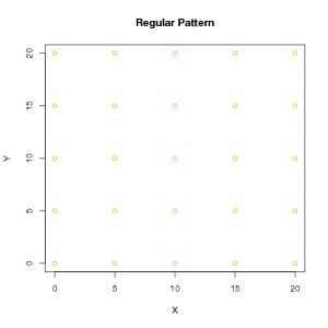
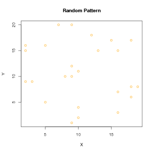
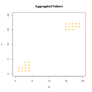
Three classifications are often used when discussing spatial patterns, aggregated (or clustered), random, and regular. These patterns are illustrated below. These classifications are part of a continuum; statistical analysis may be necessary to describe a pattern or determine what pattern classification fits an observed pattern of interest. One measure of where a particular pattern falls along the continuum is the relationship between the population variance (ơ2) and mean (μ) for each pattern, if the analyzed variable is discrete (such as an individual plant or pathogen propagule). The mean and variance are calculated by tallying the number of events within each of a set of sampling areas, such as a sampling grid, as will be discussed in more detail later. For a regular pattern, the variance is less than the mean (ơ2<μ); for a random pattern, the variance and mean are equal (ơ2=μ); and for an aggregated pattern the variance is greater than the mean (ơ2>μ) (Campbell and Madden 1990).
Below are hypothetical point pattern graphical illustrations of these three pattern definitions and the R-code used to generate them. Each point represents an organism, for example infected trees in an orchard planted in a grid fashion, 20x20 with 400 trees in each orchard. Note that the random pattern is generated independently each time it is called, so the R-code will generate a different pattern for that example each time.
Regular Pattern Illustration
   #Create a regular pattern plot with R, where every
#   fifth tree is infected along a grid
x <- c( 0,


          5, 10, 15, 20,


          0,


          5, 10, 15, 20,


          0,


          5, 10,


          15, 20,


          0,


          5, 10, 15, 20,


          0,


          5, 10, 15, 20)
y <- c( 0,


          0,


          0,


          0,


          0,


          5,


          5,


          5,


          5,


          5, 10, 10, 10,


          10, 10, 15, 15, 15, 15, 15, 20, 20, 20, 20, 20)
      # An alternative method for creating these vectors is
x


   <-


   rep(c(0,5,10,15,20),5)
y


   <-


   sort(x)
# use help(rep) and help(order)
#    to understand these commands better
   plot(x, y,


   col='orange',


   xlab='X',


   ylab='Y',


   main='Regular Pattern',


   xlim=c(0,20),


   ylim=c(0,20)
)
Output

Click to enlarge.
Random Pattern Illustration
   # Create a random pattern illustration, where
#    randomly selected trees are infected;
# Each realization is independent so yours will
#    not appear exactly as pictured below.
   x=rep(1:20,20)
y=rep(1:20,20)
xy=cbind(x,sort(y))
random.pattern=xy[sample(nrow(xy),25,replace=F),]
   plot(random.pattern,


   xlab="X",


   ylab="Y",


   col="orange")
Output

Click to enlarge.
Aggregated Pattern Illustration
In this example of a highly aggregated pattern, all the infected trees are grouped into two clusters.
   x=rep(1:2,2)
y=rep(1:2,2)
aggregated.pattern=cbind(x,sort(y))
   x2=rep(3:4,4)
y2=rep(1:4,2)
aggregated.pattern2=cbind(x2,sort(y2))
   x3=rep(15:17,3)
y3=rep(15:17,3)
aggregated.pattern3=cbind(x3,sort(y3))
   x4=rep(18:19,2)
y4=rep(16:17,2)
aggregated.pattern4=cbind(x4,sort(y4))
   plot(aggregated.pattern,


   xlab="X",


   ylab="Y",


   main="Aggregated Pattern",


   xlim=c(0,20),


   ylim=c(0,20),


   col="orange"
)
points(aggregated.pattern2,


   col="orange")
points(aggregated.pattern3,


   col="orange")
points(aggregated.pattern4,


   col="orange")
Output

Click to enlarge.
An introduction to spatial analysis is presented through examples, many of which use the
R programming environment (Garrett
et al. 2007). We include four case studies and one advanced illustration which use spatial analysis techniques to understand how pathogens spread or what control methods could be useful. The first case study uses Pearson correlation analysis to evaluate spatial relationships between a primary and alternate host. The second case study uses Lloyd's Index of Patchiness (LIP) to measure aggregation of sclerotia in soil. The third uses linear regression, discussed by Sparks
et al. (2008) in
Ecology and epidemiology in R: Disease Progress over Time, to analyze the spread of a disease in an agricultural field. The last case study uses variograms to examine disease spread. An advanced discussion about using Beta-binomial distributions in spatial analysis of plant disease concludes this document.
We have arranged the case studies in order of difficulty, with the Beta-binomial illustration being the most advanced concept presented in this document.
Next, using Pearson correlation to analyze relationships
