Vereijssen, J., Schneider, J. H. M., Stein, A., and Jeger, M. J. 2006. Spatial pattern of Cercospora leaf spot of sugar beet in fields in long- and recently-established areas. European Journal of Plant Pathology 116:187-198.
Cercospora beticola is the causal agent of Cercospora leaf spot in sugar beet (Beta vulgaris). Cercospora beticola conidia are thought to be dispersed by both rain and wind over relatively short distances throughout the growing season. Cercospora beticola overwinters in the soil by producing pseudostromata that are a source of inoculum the following spring.
Analyzing the spatial pattern of Cercospora leaf spot in the field can contribute to the design of efficient control strategies. Vereijssen et al. (2006) mapped this disease in a field over two growing seasons to determine the pattern of disease spread. They concluded that the disease tended to spread within rows of plants more than between rows, and we illustrate the general type of analysis they performed below.
In order to determine whether the spread of a disease occurs primarily across rows, within rows, or omnidirectional (Figure 1), models can be developed to determine the extent to which the disease severity or incidence of a particular individual predicts disease severity or incidence for an adjacent individual.
Let Zt(x) denote the disease severity of a plant at week “t” at location “x”. Zt(x) for a given plant can be modeled as a function of the disease severity of its neighbors. In the within-row example (Figure 1C), the estimated Žt(x) of a plant at location “x” is the average of the values for the plants immediately above and below the plant within the row (Figure 2).
zt(x-1)=1
žt(x)=1/2(zt(x-1) + zt(x+1))=1/2(1+3)=2
zt(x+1)=3
Figure 2: The disease severity of a plant at location "x" and at time "t" can be estimated by the disease severity of adjacent plants within the same row.
In order to test for a spatial pattern within a field, the estimated Žt(x) (disease severity) values can be compared to the actual Zt(x) values. If the estimate of the level of disease on a given plant tends to be improved by including the disease severity of adjacent plants as predictors, there is a non-random spatial pattern. If the omnidirectional model (Figure 1C) best predicts levels of disease, this is evidence that there is spatial aggregation of disease and disease spreads omnidirectionally. But if the across-row model (Figure 1B) or the within-row model (Figure 1C, 2) best predicts disease severity, this suggests that the disease spreads most across rows or within rows, respectively.
One method for comparing the estimated Žt(x) (disease severity) values to the actual Zt(x) values is linear regression. This method is introduced in Ecology and Epidemiology in R: disease progress over time (Sparks et al. 2008).
Below is R code for a spatial analysis using linear regression with hypothetical data. First, input the data and put it into a matrix. Then construct a map of estimated disease severity based on the average severity of neighbors.
# Input a map of observed disease severity for 100 plants
# Matrix columns represent field crop rows
# so comparisons between matrix columns are 'across-row'
# and comparisons between matrix rows are 'within-row'
row1  <-c (1,4,2,4,1,3,0,3,2,0);
row2  <-c (1,7,3,4,2,5,1,3,3,0);
row3  <-c (2,6,4,3,1,4,2,3,4,1);
row4  <-c (1,5,4,2,1,6,1,2,5,0);
row5  <-c (1,7,4,3,1,3,3,0,6,1);
row6  <-c (0,4,3,4,0,2,5,2,7,2);
row7  <-c (0,2,2,5,2,1,4,1,5,1);
row8  <-c (1,3,1,4,0,2,6,2,6,2);
row9  <-c (1,1,0,2,0,1,3,0,6,1);
row10 <-c (0,1,0,0,0,0,1,0,5,0);
# Create a matrix, called map3, with data input above
map3 <- as.matrix(rbind(row1,row2,row3,row4,row5,
                        row6,row7,row8,row9,row10));
# Make a map of estimated disease severity values
#    based on the omnidirectional model
map4 <- matrix(0,10,10);
for(xrow in 2:9){
  for(xcol in 2:9){
    map4[xrow,xcol] <- 1/4 * (map3[xrow - 1, xcol    ] +
                              map3[xrow + 1, xcol    ] +
                              map3[xrow    , xcol - 1] +
                              map3[xrow    , xcol + 1])
  }
}
map4
Output
      [,1] [,2] [,3] [,4] [,5] [,6] [,7] [,8] [,9] [,10]
 [1,]    0 0.00 0.00 0.00 0.00 0.00 0.00 0.00 0.00     0
 [2,]    0 3.50 4.25 3.00 2.75 2.50 2.50 2.50 2.25     0
 [3,]    0 4.50 4.00 2.75 2.50 3.50 2.25 2.75 3.00     0
 [4,]    0 4.50 3.75 2.75 2.50 2.25 3.25 2.25 3.00     0
 [5,]    0 3.50 4.25 2.75 1.75 3.00 2.25 3.25 3.25     0
 [6,]    0 3.00 3.50 2.75 2.25 2.25 2.75 3.25 3.75     0
 [7,]    0 2.25 2.75 3.00 1.50 2.50 3.25 3.25 3.75     0
 [8,]    0 1.25 2.25 2.00 2.00 2.00 2.75 3.25 3.75     0
 [9,]    0 1.25 1.00 1.00 0.75 1.25 2.00 2.75 3.00     0
[10,]    0 0.00 0.00 0.00 0.00 0.00 0.00 0.00 0.00     0
Note that predictions are not included for the outermost rows and columns since the complete set of neighboring plants are not available for constructing predictions. The same set of interior plants is used for all the model analyses to make comparisons between models more direct. Next, make a map of estimated disease severity values using the across-row model.
# Make a map of estimated disease severity values
#    based on the across-row model
map5 <- matrix(0,10,10)
for(xcol in 2:9){
  for(xrow in 2:9){
    map5[xrow,xcol] <- 1/2 * (map3[xrow,xcol - 1] +
                              map3[xrow,xcol + 1])
  }
}
map5
Output
      [,1] [,2] [,3] [,4] [,5] [,6] [,7] [,8] [,9] [,10]
 [1,]    0  0.0  0.0  0.0  0.0  0.0  0.0  0.0  0.0     0
 [2,]    0  2.0  5.5  2.5  4.5  1.5  4.0  2.0  1.5     0
 [3,]    0  3.0  4.5  2.5  3.5  1.5  3.5  3.0  2.0     0
 [4,]    0  2.5  3.5  2.5  4.0  1.0  4.0  3.0  1.0     0
 [5,]    0  2.5  5.0  2.5  3.0  2.0  1.5  4.5  0.5     0
 [6,]    0  1.5  4.0  1.5  3.0  2.5  2.0  6.0  2.0     0
 [7,]    0  1.0  3.5  2.0  3.0  3.0  1.0  4.5  1.0     0
 [8,]    0  1.0  3.5  0.5  3.0  3.0  2.0  6.0  2.0     0
 [9,]    0  0.5  1.5  0.0  1.5  1.5  0.5  4.5  0.5     0
[10,]    0  0.0  0.0  0.0  0.0  0.0  0.0  0.0  0.0     0
Now make a map based on the within-row model.
# Make a map of estimated disease severity values
#    based on the within-row model
map6 <- matrix(0,10,10)
for(xcol in 2:9){
  for(xrow in 2:9){
    map6[xrow,xcol] <- 1/2 * (map3[xrow - 1,xcol] +
                              map3[xrow + 1,xcol])
  }
}
map6
Output
      [,1] [,2] [,3] [,4] [,5] [,6] [,7] [,8] [,9] [,10]
 [1,]    0  0.0  0.0  0.0  0.0  0.0  0.0  0.0  0.0     0
 [2,]    0  5.0  3.0  3.5  1.0  3.5  1.0  3.0  3.0     0
 [3,]    0  6.0  3.5  3.0  1.5  5.5  1.0  2.5  4.0     0
 [4,]    0  6.5  4.0  3.0  1.0  3.5  2.5  1.5  5.0     0
 [5,]    0  4.5  3.5  3.0  0.5  4.0  3.0  2.0  6.0     0
 [6,]    0  4.5  3.0  4.0  1.5  2.0  3.5  0.5  5.5     0
 [7,]    0  3.5  2.0  4.0  0.0  2.0  5.5  2.0  6.5     0
 [8,]    0  1.5  1.0  3.5  1.0  1.0  3.5  0.5  5.5     0
 [9,]    0  2.0  0.5  2.0  0.0  1.0  3.5  1.0  5.5     0
[10,]    0  0.0  0.0  0.0  0.0  0.0  0.0  0.0  0.0     0
Creating arrays to compare severity
Observed Severity
Now make a vector of the observed severity values for the inner plants.
# Make an array of the actual disease severity values
actualo <- c(1:64)
n <- 1
for(xcol in 2:9){
  for(xrow in 2:9){
    actualo[n] <- map3[xrow,xcol];
    n <- n + 1
  }
}
actualo
Output
[1] 7 6 5 7 4 2 3 1 3 4 4 4 3 2 1 0 4 3 2 3 4 5 4 2 2 1 1 1 0 2 0 0 5 4 6 3 2 1
[39] 2 1 1 2 1 3 5 4 6 3 3 3 2 0 2 1 2 0 3 4 5 6 7 5 6 6
Estimated Values
Create arrays to compare estimated values, starting with the omni-directional model.
# Make an array of the estimated disease severity values
#    based on the omni-directional model
omni <- c(1:64)
n <- 1
for(xcol in 2:9){
  for(xrow in 2:9){
    omni[n] <- map4[xrow,xcol];
    n <- n + 1
  }
}
omni
Output
 [1] 3.50 4.50 4.50 3.50 3.00 2.25 1.25 1.25 4.25 4.00 3.75 4.25 3.50 2.75 2.25
[16] 1.00 3.00 2.75 2.75 2.75 2.75 3.00 2.00 1.00 2.75 2.50 2.50 1.75 2.25 1.50
[31] 2.00 0.75 2.50 3.50 2.25 3.00 2.25 2.50 2.00 1.25 2.50 2.25 3.25 2.25 2.75
[46] 3.25 2.75 2.00 2.50 2.75 2.25 3.25 3.25 3.25 3.25 2.75 2.25 3.00 3.00 3.25
[61] 3.75 3.75 3.75 3.00
Create an array of estimated disease severity based on across-row model.
# Make an array of the estimated disease severity values
#   based on the across-row model
across <- c(1:64)
n <- 1
for(xcol in 2:9){
  for(xrow in 2:9){
    across[n] <- map5[xrow,xcol];
    n <- n + 1
  }
}
across
Output
 [1] 2.0 3.0 2.5 2.5 1.5 1.0 1.0 0.5 5.5 4.5 3.5 5.0 4.0 3.5 3.5 1.5 2.5 2.5 2.5
[20] 2.5 1.5 2.0 0.5 0.0 4.5 3.5 4.0 3.0 3.0 3.0 3.0 1.5 1.5 1.5 1.0 2.0 2.5 3.0
[39] 3.0 1.5 4.0 3.5 4.0 1.5 2.0 1.0 2.0 0.5 2.0 3.0 3.0 4.5 6.0 4.5 6.0 4.5 1.5
[58] 2.0 1.0 0.5 2.0 1.0 2.0 0.5
Make an array of estimated values based on within-row model.
# Make an array of the estimated disease severity values
#    based on the within-row model
within <- c(1:64)
n <- 1
for(xcol in 2:9){
  for(xrow in 2:9){
    within[n] <- map6[xrow,xcol];
    n <- n + 1
  }
}
within
Output
 [1] 5.0 6.0 6.5 4.5 4.5 3.5 1.5 2.0 3.0 3.5 4.0 3.5 3.0 2.0 1.0 0.5 3.5 3.0 3.0
[20] 3.0 4.0 4.0 3.5 2.0 1.0 1.5 1.0 0.5 1.5 0.0 1.0 0.0 3.5 5.5 3.5 4.0 2.0 2.0
[39] 1.0 1.0 1.0 1.0 2.5 3.0 3.5 5.5 3.5 3.5 3.0 2.5 1.5 2.0 0.5 2.0 0.5 1.0 3.0
[58] 4.0 5.0 6.0 5.5 6.5 5.5 5.5
Linear Regression Analysis
Now that we have constructed the arrays we will use linear regression to compare observed disease severity values to the estimates from each model, beginning with the omnidirectional estimates. We are using linear regression in this application to compare the relative goodness-of-fit of the different predictive models. If we were interested in careful evaluation of p-values, we would develop a more complicated analysis that accounted for correlation between estimated values.
# Run a linear regression comparing the actual disease
# severity values to the omnidirectional estimates
roller <- as.data.frame(cbind(actualo,omni))
roller.lm <- lm(actualo~omni, data=roller);
summary(roller.lm)
Output for the omnidirectional model
Call:
lm(formula = actualo ~ omni, data = roller)
Residuals:
    Min      1Q  Median      3Q     Max
 -3.6939 -1.0562 -0.1212  0.9113  3.5816
Coefficients:
            Estimate Std. Error t value Pr(>|t|)
(Intercept)  -0.4516     0.7033  -0.642    0.523
omni          1.2756     0.2463   5.180 2.56e-06 ***
---
Signif. codes:  0 ‘***’ 0.001 ‘**’ 0.01 ‘*’ 0.05 ‘.’ 0.1 ‘ ’ 1
Residual standard error: 1.65 on 62 degrees of freedom
Multiple R-Squared: 0.302,      Adjusted R-squared: 0.2908
F-statistic: 26.83 on 1 and 62 DF,  p-value: 2.560e-06
# Check residual vs. fitted
plot(roller.lm,which=1)
More details on linear regression analysis can be found at Sparks et al. (2008).
Output
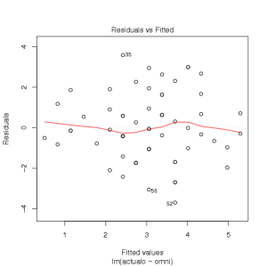
Click to enlarge.
# Check quantile-quantile plot
plot(roller.lm,which=2)
Output
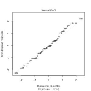
Click to enlarge.
Next, perform linear regression on the observed disease severity when compared to across-row estimates.
# Run a linear regression comparing the actual
#    disease severity values to the across-row estimates
roller <- as.data.frame(cbind(actualo,across))
roller.lm <- lm(actualo~across, data=roller)
summary(roller.lm)
Output for the across-row model
Call:
lm(formula = actualo ~ across, data = roller)
Residuals:
     Min       1Q   Median       3Q      Max
-3.56017 -1.29708 -0.06017  1.44245  3.94507
Coefficients:
            Estimate Std. Error t value Pr(>|t|)
(Intercept)   4.3180     0.4750   9.090  5.2e-13 ***
across       -0.5052     0.1632  -3.095  0.00295 **
---
Signif. codes:  0 ‘***’ 0.001 ‘**’ 0.01 ‘*’ 0.05 ‘.’ 0.1 ‘ ’ 1
Residual standard error: 1.838 on 62 degrees of freedom
Multiple R-Squared: 0.1338,     Adjusted R-squared: 0.1199
F-statistic: 9.581 on 1 and 62 DF,  p-value: 0.00295
# Check residual vs. fitted
plot(roller.lm,which=1)
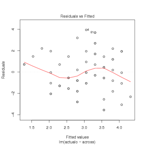
Click to enlarge.
# Check residual vs. fitted
plot(roller.lm,which=2)
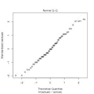
Click to enlarge.
Last compare the observed values to within-row model estimated values.
# Run a linear regression comparing the actual disease
#    severity values to the within-row estimates
roller <- as.data.frame(cbind(actualo,within))
roller.lm <- lm(actualo~within, data=roller)
summary(roller.lm)
Output for the within-row model
Call:
lm(formula = actualo ~ within, data = roller)
Residuals:
    Min      1Q  Median      3Q     Max
-2.1661 -0.7063 -0.1126  0.5212  2.4677
Coefficients:
            Estimate Std. Error t value Pr(>|t|)
(Intercept)  0.27318    0.26682   1.024     0.31
within       0.94647    0.07888  11.998   <2e-16 ***
---
Signif. codes:  0 ‘***’ 0.001 ‘**’ 0.01 ‘*’ 0.05 ‘.’ 0.1 ‘ ’ 1
Residual standard error: 1.084 on 62 degrees of freedom
Multiple R-Squared: 0.699,      Adjusted R-squared: 0.6941
F-statistic:   144 on 1 and 62 DF,  p-value: < 2.2e-16
#Check residual vs. fitted
plot(roller.lm,which=1)
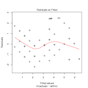
Click to enlarge.
#Check residual vs. fitted
plot(roller.lm,which=2)
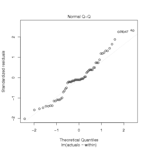
Click to enlarge.
The results of the above R code include R2 values for the three different models derived from the linear regression. Table 1 displays the R2 values taken from the above data and code.
Table 1: R2 values derived from the provided data and code demonstrating the usefulness of the various models
| Model |
R2 |
| Omnidirectional |
0.2908 |
| Across-row |
0.1199 |
| Within-row |
0.6941 |
The within-row model explains much of the variation in the data. Particularly of note, the across-row model did not identify a relationship between the disease severity of adjacent plants across rows, whereas the within-row model did identify a relationship between adjacent plants within rows. Therefore, the data suggest that the disease spreads primarily within rows of plants. This may be due to limited dispersal of infective propagules produced by the pathogen. This analysis indicates that wider spacing between susceptible plants within rows could help to slow spread of the disease.
Next, using variograms to study spatial patterns
