Throughout the exercises in dispersal, the focus has been on examining and comparing the mechanisms and assumptions that would lead to approximate exponential or power law distribution, or related distributions of propagules or disease as a function of distance from source. We can also study dispersal by asking questions that pertain to the source of inoculum. For instance, when would the starting distribution of infections be random? The distribution of initial infection is a function of the type of inoculum that initiates an epidemic. If infested seed is the source of initial infection, this would result in a random distribution to the extent that infested seed is randomly mixed with clean seed. If aerial dispersal of propagules into a field initiates the epidemic, the resulting distribution would tend to be approximately random if propagules have moved a substantial distance from the original source. By contrast, if the source of propagules is an adjacent field, propagules will tend to be deposited more heavily near that field. The distribution of infection will also differ from random, even if the distribution of propagules is random, when the biotic and abiotic environment is not homogeneous. For example, if some areas of a field are wetter, these patches will favor infection for many types of pathogens. Also, if different genotypes or species are planted across the field, such that there are different levels of resistance present, infection may be patchy.
Such concepts about dispersal can be studied via simulation. In the R code that follows, dispersal within a field will be explored, beginning with the case of random positioning of initial infections. First, a simple model of disease spread will be considered. For these exercises, we recommend that you work through this section-by-section, especially spending time to understand what the R code does. The information presented in this section on dispersal also provides an introduction to how exploration of disease processes may be handled through spatial statistics (Sparks et al. (2008).
To begin, suppose you would like to generate a simulated map of individual plants and their infection status, where infections are randomly assigned to individuals in the initial map and the number of infections per individual is tallied. One way to do this in R is as follows. Check out the contents of the different objects along the way. Use the help(sample) command to understand the sample function better.
# First generate a matrix of dimension 10x10 containing
#   zeroes, where zero indicates no infection
map1 <- matrix(0,10,10)

# Randomly select row and column coordinates for n1 initial
#   infections, where n1 can be assigned any value
n1 <- 3
row1 <- sample(1:10,size=n1, replace=T)
col1 <- sample(1:10, size=n1, replace=T)

# Assign the infections to the plants corresponding to the
#   randomly drawn coordinates, and look at the new map
for(j in 1:n1) {
  map1[row1[j],col1[j]] <- map1[row1[j],col1[j]] + 1}
map1
For example, here is one representation of three initial randomly infected plants:
map1

       [,1] [,2] [,3] [,4] [,5] [,6] [,7] [,8] [,9] [,10]
 [1,]    0    0    0    0    0    0    0    0    1     0
 [2,]    0    0    0    0    0    0    0    1    0     0
 [3,]    0    0    0    0    0    0    1    0    0     0
 [4,]    0    0    0    0    0    0    0    0    0     0
 [5,]    0    0    0    0    0    0    0    0    0     0
 [6,]    0    0    0    0    0    0    0    0    0     0
 [7,]    0    0    0    0    0    0    0    0    0     0
 [8,]    0    0    0    0    0    0    0    0    0     0
 [9,]    0    0    0    0    0    0    0    0    0     0
[10,]    0    0    0    0    0    0    0    0    0     0
Suggested exercise
Repeat this step a few times each for different values of n1, the initial number of infections, to get a feel for the appearance of a random distribution of infection. If you pick very large numbers of n1, the results may start to become unrealistic for many host-pathogen systems because host tissue would become limiting.
As a first step to modeling dispersal of pathogens, you might consider even simpler functions to describe the dispersal gradient than the exponential and power law models. Suppose we start with a scenario much simpler than dispersal following some probability distribution. For most dispersal modeling, nearer dispersal is more likely and distant dispersal is less likely. Instead, suppose that pathogens always disperse in equal numbers to the plants directly adjacent to an infected plant on a square grid. This is sometimes described as one "rook's move", with reference to the moves possible for the chess piece.
To consider this type of movement, start by generating a map of a small number of initial infections using the method above to generate map1.
Next simulate one generation of pathogen reproduction and dispersal. The following simulation has five successful propagules produced for each existing infection and one of these disperses one step to the north, one disperses one step to the south, one disperses one step to the east, one disperses one step to the west, and one infects the same host. Note that following this method, some pathogen propagules will effectively be lost off the edge of the map.
map2 <- map1
for(xrow in 1:10){
  for(xcol in 1:10){
    numprop <- map1[xrow,xcol]
    if(xrow > 1){
      map2[xrow-1,xcol] <- map2[xrow-1,xcol] + numprop}
    if(xrow < 10){
      map2[xrow+1,xcol] <- map2[xrow+1,xcol] + numprop}
    if(xcol < 10){
      map2[xrow,xcol+1] <- map2[xrow,xcol+1] + numprop}
    if(xcol > 1){
      map2[xrow,xcol-1] <- map2[xrow,xcol-1] + numprop}
    map2[xrow,xcol] <- map2[xrow,xcol] + numprop
  }
}
#See what map2 looks like now

map2
Here is an example of map2 for one set of randomly generated initial infection locations.
      [,1] [,2] [,3] [,4] [,5] [,6] [,7] [,8] [,9] [,10]
 [1,]    0    0    0    0    0    0    0    2    2     1
 [2,]    0    0    0    0    0    0    2    2    2     0
 [3,]    0    0    0    0    0    1    2    2    0     0
 [4,]    0    0    0    0    0    0    1    0    0     0
 [5,]    0    0    0    0    0    0    0    0    0     0
 [6,]    0    0    0    0    0    0    0    0    0     0
 [7,]    0    0    0    0    0    0    0    0    0     0
 [8,]    0    0    0    0    0    0    0    0    0     0
 [9,]    0    0    0    0    0    0    0    0    0     0
[10,]    0    0    0    0    0    0    0    0    0     0
To simulate n2 generations of dispersal, try the following. This also relies on having map1 generated as above with a small number of initial infections. Check out the objects created in each step (for each step that is not within a loop). Note that this is essentially the same set of commands as the example for the creation of map2, but executed n2 - 1 times.
#Assign the number of generations of
#   dispersal to be studied, n2
n2 <- 5

#Set up mapn as a list that includes n2 maps
mapn <- as.list(1:n2)

#Initialize each of the n2 maps to contain zeroes
for(j in 1:n2){mapnj <- matrix(0,10,10)}

#For each of the next maps
mapn[[1]] <- map1
for(j in 2:n2){
  #Temporarily make the map the same as one generation back
  mapnj <- mapn[[j-1]]
  #Then add the new infections following the rooks' moves
  for(xrow in 1:10){
    for(xcol in 1:10){
      numprop <- mapn[[j-1]][xrow,xcol]
      if(xrow > 1){mapnj[xrow-1,xcol] <-
        mapnj[xrow-1,xcol] + numprop}
      if(xrow < 10){mapnj [xrow+1,xcol] <-
        mapnj[xrow+1,xcol] + numprop}
      if(xcol < 10){mapnj [xrow,xcol+1] <-
        mapnj[xrow,xcol+1] + numprop}
      if(xcol > 1){mapnj [xrow,xcol-1] <-
        mapnj[xrow,xcol-1] + numprop}
      mapnj[xrow,xcol] <- mapnj[xrow,xcol] + numprop
    }
  }
}

#See what mapn looks like
mapn
Here is one example of mapn:
1
      [,1] [,2] [,3] [,4] [,5] [,6] [,7] [,8] [,9] [,10]
 [1,]    0    0    0    0    0    0    0    0    1     0
 [2,]    0    0    0    0    0    0    0    1    0     0
 [3,]    0    0    0    0    0    0    1    0    0     0
 [4,]    0    0    0    0    0    0    0    0    0     0
 [5,]    0    0    0    0    0    0    0    0    0     0
 [6,]    0    0    0    0    0    0    0    0    0     0
 [7,]    0    0    0    0    0    0    0    0    0     0
 [8,]    0    0    0    0    0    0    0    0    0     0
 [9,]    0    0    0    0    0    0    0    0    0     0
[10,]    0    0    0    0    0    0    0    0    0     0

2
      [,1] [,2] [,3] [,4] [,5] [,6] [,7] [,8] [,9] [,10]
 [1,]    0    0    0    0    0    0    0    2    2     1
 [2,]    0    0    0    0    0    0    2    2    2     0
 [3,]    0    0    0    0    0    1    2    2    0     0
 [4,]    0    0    0    0    0    0    1    0    0     0
 [5,]    0    0    0    0    0    0    0    0    0     0
 [6,]    0    0    0    0    0    0    0    0    0     0
 [7,]    0    0    0    0    0    0    0    0    0     0
 [8,]    0    0    0    0    0    0    0    0    0     0
 [9,]    0    0    0    0    0    0    0    0    0     0
[10,]    0    0    0    0    0    0    0    0    0     0

3
      [,1] [,2] [,3] [,4] [,5] [,6] [,7] [,8] [,9] [,10]
 [1,]    0    0    0    0    0    0    4    8    9     4
 [2,]    0    0    0    0    0    3    8   12    8     3
 [3,]    0    0    0    0    1    4   10    8    4     0
 [4,]    0    0    0    0    0    2    4    3    0     0
 [5,]    0    0    0    0    0    0    1    0    0     0
 [6,]    0    0    0    0    0    0    0    0    0     0
 [7,]    0    0    0    0    0    0    0    0    0     0
 [8,]    0    0    0    0    0    0    0    0    0     0
 [9,]    0    0    0    0    0    0    0    0    0     0
[10,]    0    0    0    0    0    0    0    0    0     0

4
      [,1] [,2] [,3] [,4] [,5] [,6] [,7] [,8] [,9] [,10]
 [1,]    0    0    0    0    0    7   24   41   38    20
 [2,]    0    0    0    0    4   18   45   56   44    18
 [3,]    0    0    0    1    6   24   44   45   24     7
 [4,]    0    0    0    0    3   12   24   18    7     0
 [5,]    0    0    0    0    0    3    6    4    0     0
 [6,]    0    0    0    0    0    0    1    0    0     0
 [7,]    0    0    0    0    0    0    0    0    0     0
 [8,]    0    0    0    0    0    0    0    0    0     0
 [9,]    0    0    0    0    0    0    0    0    0     0
[10,]    0    0    0    0    0    0    0    0    0     0

5
      [,1] [,2] [,3] [,4] [,5] [,6] [,7] [,8] [,9] [,10]
 [1,]    0    0    0    0   11   56  141  200  181    96
 [2,]    0    0    0    5   32  116  232  287  224   107
 [3,]    0    0    1    8   44  128  226  232  151    56
 [4,]    0    0    0    4   24   78  128  116   56    14
 [5,]    0    0    0    0    6   24   44   32   11     0
 [6,]    0    0    0    0    0    4    8    5    0     0
 [7,]    0    0    0    0    0    0    1    0    0     0
 [8,]    0    0    0    0    0    0    0    0    0     0
 [9,]    0    0    0    0    0    0    0    0    0     0
[10,]    0    0    0    0    0    0    0    0    0     0
The output mapn is a list in which each matrix is a map after a new generation of dispersal.
Suggested exercise
Try this for a series of different initial maps generated as map1. To do this, you could cut and paste the material from above when needed. Alternatively, you could create a function that performs these steps, as below.
disperse <- function(map1,n2){
  mapn <- as.list(1:n2)
  for(j in 1:n2){mapnj <- matrix(0,10,10)}
  mapn[[1]] <- map1
  for(j in 2:n2){
    mapnj <- mapn[[j-1]]
    for(xrow in 1:10){
      for(xcol in 1:10){
        numprop <- mapn[[j-1]][xrow,xcol]
        if(xrow > 1){
          mapnj[xrow-1,xcol] <-
              mapnj[xrow-1,xcol] + numprop}
        if(xrow < 10){
          mapnj [xrow+1,xcol] <-
              mapnj[xrow+1,xcol] + numprop}
        if(xcol < 10){
          mapnj [xrow,xcol+1] <-
              mapnj[xrow,xcol+1] + numprop}
        if(xcol > 1){
          mapnj [xrow,xcol-1] <-
              mapnj[xrow,xcol-1] + numprop}
        mapnj[xrow,xcol] <-
            mapnj[xrow,xcol] + numprop
      }
    }
  }
  mapn
}
You could use this function as in the following examples (which assume you have a matrix map1 already created). You could try this command after generating different versions of map1 to compare the patterns.
disperse(map1,n2=3)
disperse(map1,n2=5)
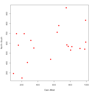
In the above examples, locations were randomly selected individual hosts where the number of infections was tallied. It might be more realistic to consider a situation where the initial infections are randomly applied to a continuous map. That is, nstart infections are assigned to continuous x and y coordinates in a 1000 m by 1000 m map. The random assignment is performed using the runif function. This function generates random numbers with a uniform distribution across the range requested. Try help(runif) for more information.
#Assign the number of initial infections, nstart
nstart <- 20

#Randomly draw x and y coordinates for the initial infections
row1 <- runif(n=nstart, min=0, max=1000)
col1 <- runif(n=nstart, min=0, max=1000)

#Plot the initial infections
plot(row1, col1, xlab="East-West",
     ylab="North-South", pch=19, col="red")

Click on the image for larger version.
Next, suppose that each infection produces nnew new infections in the next pathogen generation. These new infections are equally likely to occur in any direction from the source infection. (When would this assumption not be reasonable?) The coordinates for a randomly-drawn direction can be generated as follows, again using the runif function, but ranging from -? to ?. Here the random variables are transformed with functions sin and cos to generate points in all possible directions from a source in two dimensions.
#Assign the new number of infections from
#   each initial infection, nnew
nnew <- 50

#Generate nnew random directions from a source
temp <- runif(n=nnew, min=-pi, max=pi)

#Plot the points in the different directions,
#   for wno equidistant from source
plot(sin(temp),cos(temp))
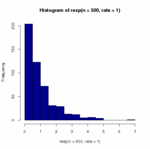
Suppose the distance from the source at which a new infection occurs is described by an exponential model. R supplies a function to generate random numbers generated from an exponential distribution, as well as the uniform distribution used above and many others (see Garrett et al. In Press). The rexp function generates random variables drawn from an exponential distribution with parameter rate. You can get a feel for how the rate parameter affects the shape of the distribution by trying the following. The hist command produces a histogram of the variables generated. If n=500 or more variables are generated, this gives a pretty clear idea of the shape of the distribution. If a small number of variables are generated, the shape is not so clear. But it is also informative to try drawing just a small number n of samples from the distribution to get a feel for what it means to "draw from a distribution".
hist(rexp(n=500, rate=1),col="blue")

Click on the image for larger version.
Now, combine the initial random map of infections, the random direction of new infections, and the exponential model describing the distance at which new infections occur. The following function is the first step for generating maps of infection for ngen generations.
# nstart is the number of initial infections
# nnew is the number of new infections produced by each
#      pre-existing infection each generation
# ngen is the number of generations
# exppar is the rate parameter for
#    the exponential distribution
disperse2 <- function(nstart, nnew, ngen, exppar){
  coord <- matrix(runif(n=2*nstart, min=0, max=1000),
             nrow=nstart, ncol=2)
  ntot <- nstart
  for(i in 1:ngen){
      for(j in 1:ntot){
        tempx <- coord[j,1]
        tempy <- coord[j,2]
        newdir <- runif(n=nnew, min=-pi, max=pi)
        newdist <- rexp(n=nnew, rate=exppar)
        newx <- tempx + newdist * sin(newdir)
        newy <- tempy + newdist * cos(newdir)
        newcoord <- cbind(newx,newy)
        coord <- rbind(coord,newcoord)
      }
   ntot <- length(coord[,1])
   }
coord
}
Try the following commands, varying the values of the input parameters. Especially try different values of the exponential paramater, exppar. More fun than a video game?
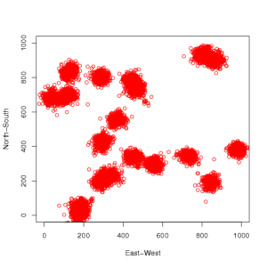
tmat <- disperse2(nstart=20, nnew=10, ngen=3, exppar=0.1)
plot(tmat, xlim=c(0,1000), ylim=c(0,1000), xlab="East-West",
     ylab="North-South", col="Red")
This leads to the following graph:
Output

Click on the image for larger version.
As a more advanced exercise, try generating different maps using R functions that generate random numbers from the related gamma and Weibull distributions, too: rgamma and rweibull. Try different values of the shape and scale parameters for both these distributions too. Here are examples to remind you of the shape of those distributions; you can change the shape parameters to plot histograms representing the different parameter combinations.
hist(rgamma(n=500, shape=1, scale=1), col="blue")
hist(rweibull(n=500, shape=1, scale=1), col="blue")
Note that there are several different ways to get similar-looking spatial patterns. In a practical application, such as trying to model a real epidemic, it may not matter greatly which of these models you use. This exercise is intended to give you an idea of some of the tools available.
Next, concluding remarks
