DisplayTitle

Bayesian Analysis with SAS

1.  There are several software packages that can perform Bayesian analysis. However, in this article, Bayesian analysis will be conducted in SAS (http://www.sas.com). The SAS software, in particular, has some procedures that are much easier to use than other programs for many common data-analytical problems (Stokes et al., 2014).

There are two general approaches to perform Bayesian analysis using SAS.

(a) With the SAS procedures GENMOD, LIFEREG, PHREG, and FMM, one can use the BAYES statement to obtain Bayesian analysis (Stokes et al., 2014). These procedures perform frequentist (or likelihood-based) analyses as a default, but the BAYES statement can be used to request a Bayesian analysis following the frequentist analysis using Gibbs sampling (or other MCMC sampling algorithms, with the default sampling method depending on the distribution of the data and model type).

Example:

proc genmod;
   model y = x1 x2 x3    /*x1, x2, x3 are explanatory variables*/
            / dist=binomial link=logit;
   bayes;
run;

This is an example of a logistic regression analysis with three predictor variables (x1, x2, x3), where a logit link function is linearly related to the predictors. The procedure first determines the maximum likelihood estimates of the parameters (intercept, and θ coefficients for x1, x2, and x3), and then uses these estimates as starting points for the sampling of the posterior.

The default prior distribution for these fixed-effect parameters is the uniform distribution. However, GENMOD uses a special kind of uniform distribution, one in which the value of the distribution (i.e., density function) is 1 at all values of the parameters (see Fig. 2B). This is known as an improper prior distribution because when a true (i.e., proper) distribution is integrated over all values, the result is a value = 1. With an improper distribution, the integration across all values results in a value that is greater than 1 (and usually equal to infinity). Interestingly, this is not a problem when applying Bayes’ Theorem to data analysis because the P(y) constant in the denominator of equation 4 is also rescaled accordingly, so that the posterior is a proper distribution.

Figure 2. Examples of non-informative prior distributions. (A) uniform, (B) constant, or flat such as “1”, and (C) normal distribution N(m,v) where m is the mean and v is the variance; when variance is very large, ie., 10⁶ then normal is similar to uniform (blue line). Click to enlarge.

One can change the prior distribution for the parameters to a normal distribution with the following statement:

bayes coefprior=normal;

The default variance (v) of the prior is 10⁶, so clearly this is a noninformative prior. Interestingly or surprisingly, GENMOD displays the inverse of this variance in the output with the label of Precision (Precision = 1/v = 10^-6). Bayesians often like to express certainty as precision rather than as the variance (or standard deviation).

Below are options that are available in all four procedures:

INITIAL = specifies initial values of the chain
NBI = specifies the number of burn-in iterations
NMC = specifies the number of iterations after burn-in
SEED = specifies the random number generator seed
THINNING = controls the thinning of the Markov chain
DIAGNOSTICS = displays convergence diagnostics

There are also other OPTIONS specific to each of the four PROC that can be found in the SAS/STAT User’s Guide. Some of these options are described in this paper below. 

(b) PROC MCMC, which uses one of several MCMC sampling methods (e.g., Metropolis-Hastings) (Chen, 2009), is essentially a full programming language, where one specifies the likelihood function for the data and prior distributions for the parameters, and other aspects of the model fit. This PROC enables you to analyze data that have any likelihood or prior distribution. On the other hand, it requires advanced computational skills. We demonstrate a simple version of the program syntax here for the logistic regression problem mentioned above, but this paper is not an appropriate place to teach the programming language of the procedure. 

Example:  

proc mcmc seed=28513;
parms beta0 0 beta1 0 beta2 1 beta3 1;
prior beta: ~ normal (mean=0, var=1e6); *-all the priors have noninformative normal distributions;
p = logistic(beta0 + beta1*x1 + beta2*x2 + beta3*x3);
model y ~ binomial(p);
run;

The PARMS, PRIOR, and MODEL statements form the basis of every Bayesian model developed using PROC MCMC. Every parameter in the PARMS statement, which defines the parameters of the model, must have a corresponding prior distribution in the PRIOR statement. The OPTIONS mentioned before are available also with the PROC MCMC along with a few more:

DIC = computes and displays deviance information criterion (DIC)
MONITOR = analysis for selected parameters of interest
AUTOCORLAG = specifies the number of autocorrelation lags used to compute effective sample sizes and Monte Carlo errors.

There are also other OPTIONS that can be found in the SAS/STAT User’s Guide.

2. Diagnostic Criteria

Convergence

Convergence of the Markov chain is important for inference, but it can be a difficult concept to understand. There are many iterative methods in statistics that need to converge, but convergence is to a point (e.g., a point estimate in a frequentist analysis of a nonlinear model). In Bayesian analysis, however, convergence is to a distribution, to the extent that even after convergence, each iteration will give a different sampled valued. There is no single unambiguous way to assess convergence, but there are several helpful tools to evaluate convergence of the algorithm. Assessment of convergence requires a few steps. One needs to decide if the Markov chain has reached stationary stage; then one should decide on the number of iterations to keep after the Markov chain has reached stationarity (samples collected before convergence to stationarity are usually discarded). The samples kept are then used to derive the values of parameters of interest of the posterior distribution.

Procedures such as GENMOD usually discards a fixed number of MCMC samples at the start of the process and keeps the rest. The first phase of the sampling process is known as the burn-in period. The default period in GENMOD is 2,000 but this can be easily changed (typically, increased) with the NBI (“number of burn-in iterations)” option.  By default, GENMOD samples 10,000 parameter values, which is adequate for many problems but the samples can be increased with the NMC option described above. After the burn-in, the procedure uses all of the remaining samples (as a default) to estimate the posterior. However, this is fully valid only if there is no correlation in the MCMC samples. A high correlation between a sampled posterior observation and previous samples can be problematic, but there is a solution to avoid this issue.

Thinning is the practice of keeping every i-th simulated draw from a chain, instead of every draw, so that the sample autocorrelation of the final sample used to construct the posterior is reduced. High autocorrelation is an indication of poor sampling efficiency. If there is evidence that each sample is highly correlated with the previous two samples, then one could use THINNING=2 in GENMOD, so that the procedure uses every third MCMC sample. Thinning results in wasting samples of the posterior distribution. The posterior distribution always is expected to be more precise if all samples are used. If heavy thinning is used, then the number of MCMC samples (NMC) should be increased, and possibly substantially, so that there are at least 10,000 samples used in the analysis.

Before deciding on whether the algorithm has converged, one should check the posterior distributions of all parameters and not only a few. Even if the posterior distributions of some parameters appear to have converged, posterior distributions of some other parameters may not have converged. In such cases one cannot simply assume good convergence even for parameters that appear to have converged.

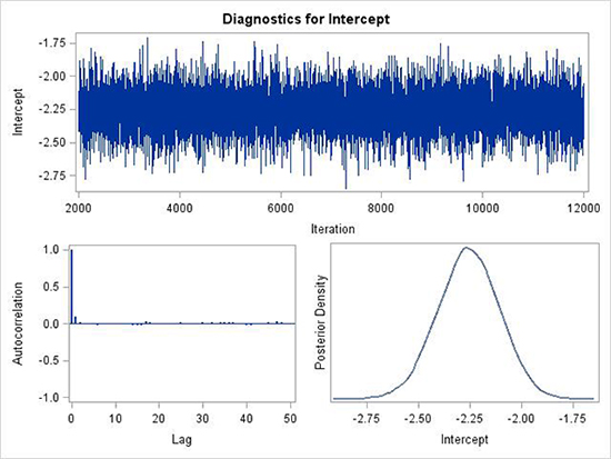
Below are three examples of important diagnostic plots automatically produced by GENMOD (and by other procedures in SAS) (Fig. 4, 5 and 6).  These three plots are produced for each parameter in the model. Results for the intercept parameter is shown in Fig. 4 and 5. In each figure there are 3 sub-plots: trace plot, autocorrelation plot and posterior density plot. In Fig. 4, the first plot is the trace plot, a sequential graph of all the MCMC samples in the chain. Note that the first sample starts at 2000 because the burn-in was 2000 (default). There are then another 10,000 samples generated. The trace plot in Fig. 4 is the ideal that one should be looking forward for. There is no trend, and the values jump randomly above and below the central value. The autocorrelation plot shows the serial correlation of each sample in the chain with the previous samples; lag 1 is for each sample with the previous one, lag 2 is for each sample with the one two samples previously, and so on. At lag 0, the autocorrelation is 1, by definition, but is shown to provide perspective in interpretation. In Fig. 4, the lag 1 correlation is very close to 0, and the remaining correlations are even closer to 0. This is ideal.  Finally, the posterior density plot is an estimate of the posterior distribution based on the 10,000 samples used from the trace plot (Fig. 4). A kernel smoothing algorithm is applied to the values to produce the curve. This posterior density is the ultimate goal of the Bayesian analysis. Summary statistics are derived from the samples that comprise the empirical density, such as the mean, median, standard deviation, and so on (see examples, below). It should be noted that the standard deviation of posterior density is analogous to the standard error in frequentist analysis.

Figure 4. Example of good mixing of the MCMC samples for the posterior distribution of a parameter. Autocorrelations are low, trace plot does not demonstrate a trend, and posterior density is very smooth.
Click to enlarge.

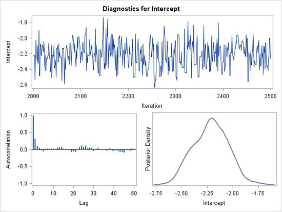
Figure 5 shows an example that is slightly less than ideal. First, note that only 500 samples are generated in this example after the 2,000 burn-in samples and as such, the values are less crowded. One can see that the samples do not simply jump randomly around a central value, but sometimes move a bit slowly above and below the center value. There are times where the samples tend to be high (or low) for several samples in a row. The lag-1 autocorrelation is moderate (about 0.3), with smaller correlations after that. This is an example where THINNING=1 will take care of the lag-1 autocorrelation and every other sample is kept to calculate the posterior distribution. It should be noted that with difficult model fitting problems, it may be difficult to get better mixing than shown in this figure. 

Figure 5. Example of less than ideal mixing of the MCMC samples for a posterior distribution of a parameter. There is evidence of autocorrelations, trace plot does not jump randomly, and posterior density is not very smooth. Click to enlarge.

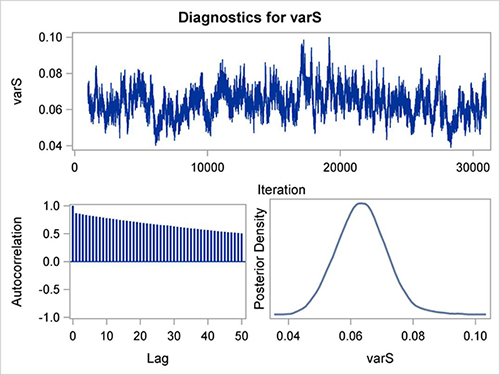
Figure 6 is an example of very poor mixing in the MCMC chain. This is an example from a nested model (with multiple random effects) fitted by PROC MCMC (beyond the scope of this article). The autocorrelations are high and decline very slowly. The trace plot shows very slow movement of the parameter values above and below the central value. This is a totally unacceptable sampling, and these results cannot be used since they indicate a poor model. Thinning could potentially be used to improve convergence but it would have to be extreme (say, THINNING=70), where very few generated samples are used and this would require very large numbers of generated samples. In such a case, other approaches should be used to satisfy the Bayesian assumptions and these alternative approaches could include using a different model, choosing different variables in the model, choosing a different prior, or selecting a different MCMC sampling algorithm. These remedies are beyond the subject of this paper and will not be discussed here. Fortunately, the Bayesian analysis using GENMOD usually do not lead to difficulties outlined above.

Figure 6. Example of very poor mixing of the MCMC samples for a posterior distribution of a parameter. The autocorrelations are high and decline very slowly, whereas the trace plot shows very slow movement.
Click to enlarge.

Procedures in SAS also provide, as default or as options, several statistical measures of model fit, especially for convergence to the target posterior distribution. These include the following.

i) Geweke Diagnostics compares values in the early part of the Markov chain with those in the latter part of the chain to detect failure of convergence. If the ratio of values is close to 1 then convergence is good. (Geweke, 1992). 

ii) Effective sample size is a measure of how well a Markov chain is mixing. An effective sample size substantially lower than the actual sample size shows slow or poor mixing of the Markov chain. Usually visual inspection of the trace plots (as shown above) is the most useful criterion.

iii) Deviance Information Criterion (DIC)
A criterion called the DIC (Deviance Information Criterion) is the Bayesian version or generalization of the well-known AIC (Akaike Information Criterion). The DIC was proposed by Spiegelhalter et al. (1998, 2002). One of the major advantages of the DIC is that it can be easily calculated when using Markov Chain Monte Carlo (MCMC) simulation. The DIC can be used to select models with better predictive ability and lower complexity.

The basic idea is to estimate the error that would be expected when applying the model to future data. The DIC is based on a trade-off between the fit of the data to the model and the number of parameters (w) in the model. In a manner that is analogous to the classical AIC, DIC is defined as:

where y is the data, the average of the unknown parameters q, D the deviance and  the average deviance. The DIC is displayed by GENMOD (using “p” for w in the output).

Examples:

We will examine the examples used in Chapter 15 of the “Exercises in Plant Disease Epidemiology, 2nd edition” (Mila and Yuen, 2015), plus one other example. Bayesian analysis in that chapter was performed with OpenBugs, a statistical package specialized in Bayesian analysis using Gibbs sampling. OpenBugs requires some understanding and expertise in writing the programming code. Here the analysis will be conducted with SAS version 9.3. For readers that have access to both SAS and OpenBugs, this example gives them the opportunity to compare the Bayesian analysis done using two different computational packages. 

We will examine five simple case studies. The first four are based on a logistic regression problem, where the fitted model is:

where X₁ represents cumulative degree days (CDD), X₂ is the total precipitation measured in mm (RAIN), X₃ is continuous days of rainfall (WW), and p is the probability of latent infection of soybean in the field (Mila et al., 2005). We do not go into the many instructions for using GENMOD for modeling; one should consult the SAS User’s Guide for these details. Stokes et al. (2014) provide many more details for Bayesian analysis using GENMOD. A supplemental SAS program file containing the data and the GENMOD code for case #1 to #4 is provided.