DisplayTitle

Case Study #5

This is a different data set from the one used above and was provided kindly by Dr. Xiangming Xu of East Malling Research Station, UK. These data were generated from a study that evaluated three treatments (including the control) on the number of powdery mildew lesions on apples grown in the greenhouse (unpublished). The supplemental SAS program file contains the data and the GENMOD code. The experiment was arranged in a completely randomized design. Although lesion counts were determined for different leaves and shoots, they were pooled to obtain the total lesions per plant. Assuming that the number of lesions per plant has a Poisson distribution, the fitted model can be written as:

ln(m_j) = t_j

where m_j is the expected value (mean) for the j-th treatment (j = 1, 2, 3), ln(.) is the log link function, and t_j is the effect of the j-th treatment on the log of the mean.

We determine the effect of treatment on lesions using the following code:

proc genmod data=apple24o;
class trt;
model lesions = trt / noint  dist=poisson  link=log ;
lsmeans trt / cl diff  plots=all;
bayes cprior=normal seed=12345;
run;

(trt) is listed in the CLASS statement (to indicate that it is a factor and not a continuous covariate as in the other examples). A Poisson distribution and log link with options on the MODEL statement is indicated here in the SAS code. The noint option tells GENMOD to fit a model without an intercept (no intercept). This way, the three parameters correspond to the three treatment means (on a log link scale). If there was an intercept, the last parameter would be 0 (by definition) and the intercept would be the mean (on a log link scale) for the last treatment. A noninformative normal prior is used here for the treatment effect parameters. The output below is from running GENMOD using SAS version 9.3. When running GENMOD in SAS version 9.4, one needs to remember to add sampling=arms option if ARMS is used for sampling. Note that an LSMEANS statement is added to obtain the posterior distributions (and associated statistics) for ln(m_j) for each treatment. The options on this statement request credible intervals for ln(m_j) (cl), and for the differences of each pair of treatment means (diff). The plots option allows the program to generate several useful graphs.

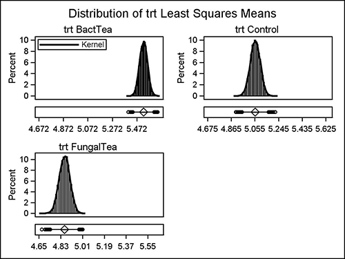
The reader can confirm that there was good mixing of the MCMC chain, with convergence for each parameter (t₁, etc.). The LSMEANS statement also allows one to obtain the posterior distribution of the means (on the log scale) (Fig. 9). On can also see box plots for these posteriors (plotted in a horizontal manner) underneath the density plots (based on 10000 samples, the default). The scale is about the same for all three graphs, so one can easily see the different magnitudes of the means for the different treatments. The means of the posteriors and the credible intervals are displayed in Table 3.

Figure 9. Posterior distributions of ln(m1), ln(m₂), and ln(m₃) for case study 5. Click to enlarge.

Table 3. The means of the posteriors and their corresponding 95% credible intervals (analogous
to a confidence interval with frequentist analysis) for parameters in case study #5. Click to enlarge.

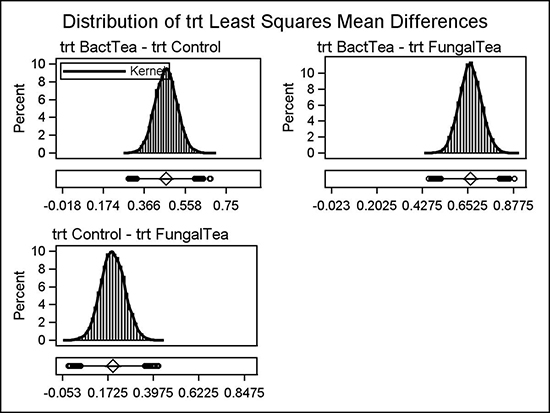
As explained above, “Estimate” is the mean of the posterior distribution (log scale). The limits of the 95% credible interval (Lower HPD and Upper HPD) are given in the last two columns. Again, the diff option allows one to also obtain posterior distribution graphs for the differences of pairs of means (on a log scale) (Fig. 10).

Figure 10. Posterior distributions of differences of means on log scale (e.g., ln(m₁) – ln(m₂), etc.),
together with Box plots (drawn horizontally) of the posteriors. Click to enlarge.

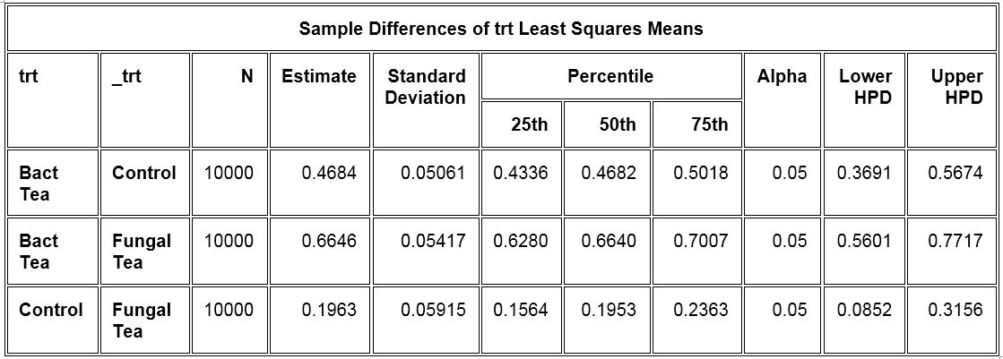
One can see that the posterior distributions of the differences mostly do not cover 0. This indicates that there are differences among the treatment effects. The greatest coverage of 0 by a posterior distribution was for the last pair of means (control versus fungal tea), although most of the posterior consisted of positive values. A table of summary statistics for the posteriors of the differences is also given in the output (Table 4).

Table 4. Summary statistics for the posteriors of the differences of case study #5. Click to enlarge.

The “Estimate” in this table is the mean of the posterior distribution for the difference of two treatments. One can see that all of the 95% credible intervals for the differences do not include 0, evidence that the treatments are different from each other.

Suggested exercises:

(a) Readers can obtain the posterior distribution of the means on the original lesion-count scale instead of on the link (log) scale. The model for a Poisson distribution should usually be fitted on a log scale, but one can obtain the posterior of the inverse link (i.e., lesion counts directly, exp[ln(m_j)] = m_j) by adding the ilink option to the LSMEANS statement:

lsmeans trt / cl diff  ilink plots=all;

The posterior graphs and means table are for m₁, etc., rather than for ln(m₁), etc. Readers should note that the posteriors of the mean differences are still given only on the link scale. This is because the inverse link of the differences of logs does not have a direct distributional interpretation.

(b) Using the methods described previously, readers should explore the effects of an informative prior distribution on the control treatment. Suppose that previous experiments showed that ln(m_control) [=ln(m₂) in this study] was 5.3, and that one was 95% confident that the log mean was between 5.0 and 5.6. Use the prior parameter file and previous code to fit the model. How do the results change for the means and for the mean differences?

(c) Record the DIC from the model fit. Then run GENMOD without the treatment factor, but with an intercept: model lesions = / dist=poisson  link=log;. Record this DIC. What is the difference in DIC for the two model fits? A large difference would indicate that treatment has an overall effect on lesion counts.