GENMOD/Bayes statement and informative priors
data Prior;
input _type_ $ CDD WW RAIN;
datalines;
Mean 0.01 0 0
Var 0.001 1e6 1e6;
run;
proc genmod data=ONFIT;
model ONFIT/N = CDD RAIN WW/ dist=binomial link=logit;
bayes seed=27500 coeffprior=normal(input=Prior)
outpost=bayes diag=all;
title 'Bayesian analysis of Latent Infection with informative normal priors';
run;
Note how one specifies the priors using coeffprior=normal(input=Prior) option in the bayes statement.
The reader can confirm the “estimates”, the posterior percentiles and HPD limits. The DIC in case #2 remained almost unchanged by the implementation of normal priors comparing to the DIC obtained in case
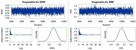
#1. Thus, one can conclude that the use of normal priors (non-informative overall, and informative for CDD) did not substantially improve the model. The mixing of the MCMC chain was still good (Fig. 8) but more lags were necessary to reduce the autocorrelation in the parameter estimation (Fig. 8).

Figure 8. MCMC chain, autocorrelation plot and posterior distributions for parameters RAIN, and WW
with non-informative normal priors (instead of the improper flat priors used in case #1).
Click to enlarge.
Suggested exercises after completing case study #2:
(a) Compare results from case study
#1 and #2. What differences in posterior distributions do you see? What differences in summary statistics (mean, standard deviation, credible interval) do you see? Some of the differences are mentioned above but the readers will gain more insight by looking at the summary tables as well.
(b) Repeat case study
#1 using only CDD and WW as input variables. Compare the DIC value with the one of case
#1. Readers need to remember that although there is no perfect value for DIC, a large DIC number indicates that there might be more parameters to include in the model that would lead in a lower DIC value. The smaller the DIC value, the better the model.
(c) Repeat case study #2 implementing informative priors of your choice on parameter estimates for variables
WW and
RAIN. Note that you have to run the Prior data step
and the GENMOD procedure to get the new priors. Compare the results. Try a range of prior distribution variances and means for the parameters, using the range95 rule-of-thumb described above in selecting the size of the variance. Comment on the change in the results, if any.
(d) Repeat case study #2 by changing THINNING to 10 and compare results with case study #2. As a reminder, THINNING helps with good MCMC chain mixing and reduces the autocorrelation. In case study #2, autocorrelation did not drop fast within the first few lags; thus, using THINNING may help in reducing autocorrelation. We urge the readers to check the autocorrelation plots before and after implementing THINNING.
The following are demonstrations on the use of more difficult, but more general (and flexible), MCMC procedure. Detailed programming description for this procedure is beyond the scope of this chapter, but it is helpful to see its operation here.
