GENMOD/Bayes statement and flat (uniform) non-informative priors
proc genmod;
model ONFIT/N = CDD RAIN WW/ dist=binomial link=logit;
bayes seed=27500;
title 'Bayesian analysis of Latent Infection with non-informative priors';
run;
Note that ONFIT is the response variable (the number with latent infection, which has a binomial distribution, and
N is the number observed). As explained above, the seed option assures that one obtains the exact same answer every time the program is run. One should note that the seed option is not usually required when implementing GENMOD. The simple use of the BAYES statement gives an improper flat prior (the default) for each of the θ parameters. A SEED option is given so that the exact same samples are obtained from the posterior each time the procedure is run; this is useful for educational purposes. The seed option can usually be omitted.
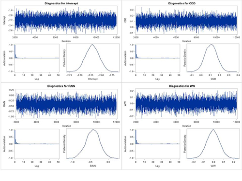
Based on the diagnostics, there was a good mixing of the MCMC chain, with convergence for each parameter (CDD, RAIN, WW, and intercept). Autocorrelation dropped quickly within a few lags and posterior distributions of all parameters seem smooth (Fig. 7).

Figure 7. MCMC chain, autocorrelation plot and posterior distributions for intercept, CDD, RAIN,
and WW with case study #1.
Click to enlarge.
In Table 1, “estimate” is the mean of the posterior distribution for each parameter. There is more than one way to calculate the credible interval, and GENMOD displays results for the two most common approaches. The HPD (highest posterior density) method may be the more accurate approach, and we show that result here. Percentiles and HPD are extensively used in Bayesian methods to make inference about parameter estimates. For instance in this case, the 25% and 75% percentiles for intercept, CDD and RAIN are in the negative, positive and negative space, respectively, while those for WW are in both the negative and positive space. In other words, the posterior distribution for WW includes 0, an indication that WW may not be a significant explanatory parameter. The complete SAS output for case #1 is given in the supplemental file named “Output_Case1”, where, also, the different components of the output are explained in a greater detail.

Table 1. The means of the posteriors and their corresponding 95% credible intervals (analogous to a confidence interval with frequentist analysis) for parameters in case study #1.
Click to enlarge.
The statement
bayes seed=27500 coeffprior=normal;
can be used for a normal non-informative prior for each parameter (i.e., normal distribution with a very large variance).
The default MCMC sampling algorithm in GENMOD for a binomial (or Poisson) distribution changed between versions 9.3 to 9.4 of SAS. In 9.3, ARMS sampling (a version of Gibbs sampling) is used, while Gamerman sampling is used in version 9.4. Differences in the sampling method used can lead to slightly different numerical results but not the overall significance of the model. The output in this paper was generated in SAS version 9.3. Individuals who use 9.4 can obtain ARMS sampling (and thus, directly obtain the same output as in this paper) by adding a sampling option to the BAYES statement:
bayes seed=27500 coeffprior=normal
sampling=arms;
Conversely, if a user of version 9.3 wishes to use Gamerman sampling, this can be achieved using the following statement:
bayes seed=27500 coeffprior=normal
sampling=gamerman;
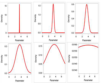
GENMOD only allows the normal distribution to be used for informative priors. In contrast, procedures such as MCMC allow for a wide range of possible prior distributions. GENMOD may seem overly restrictive, but this is not really a limitation for many (or most) data analyses. As shown above (Fig. 3), the normal distribution can be used for very informative to non-informative priors, all based on the variance (and mean) of the distribution. To use an informative prior with GENMOD, one must specify the mean and variance of the normal prior for each parameter in a separate file, and then reference this file when running GENMOD. The special file (called Prior in case study
#2) has two records, the first record for the mean and the second record for the variance of the prior. The records must start with ‘Mean’ and ‘Var’, respectively. There is a column (variable) that identifies the record
(_type_) and a column for each of the terms in the model being fitted. For the example here, we use non-informative priors for the parameters for WW and RAIN (v = 106) and a very informative prior for the parameter for CDD (v = 0.001 and mean = 0.01).

Figure 3. Normal distributions with increasing variances (0.000625, 0.0625, 0.25, 1.56, 6.25, 625.0). Note the flattening of the curve with increasing variance.
Click to enlarge.
Annotated Output PDF
Data and Code SAS File
